
AI learns to sail upwind
Solving sailing using Q-Learning

The year 2020 was not the greatest for sailors. The pandemic limited the available options for voyages or even to gather a crew. I am a huge sailing enthusiast and I felt a big hole in my heart, not having the opportunity to pursue my passion. That’s when I thought that I could at least let my computer go sailing and train it the basics of yachting.
The code for this project is available on Github.
You can see the agent learn to solve two different tasks in the demos below. Click the button to start the simulation, the button to speed through a number of episodes and the to start over. The whole training process is explained later.
Open Sea
An agent learns to sail as far north as possible. There are no limitations, so it converges to a direction, which gives the best speed in the northern direction.
Read More
Modelling the effect of wind
We will move on to the model of the wind. Since sailboats are powered by the wind it will be sufficient to focus on the effect the wind has on the velocity of the boat. I assume that the agent knows how to trim the sails appropriately and how to execute the technicalities of manoeuvres like tacking (crossing the line of wind). This means that we assume that for the given angles against the wind, we are obtaining the best possible velocity. There are a few features that we need to keep in mind.
- The direction of the wind $\theta_0$ and that you cannot sail directly upwind.
- The dead zone of the boat $\theta_{dead}$, where the sailboat loses a significant amount of speed
- The maximal velocity obtainable under the given wind $V_0$.
Therefore we construct the model as a function of the boat velocity to the angle $\theta$ of the boat.
\begin{equation} V(\theta) = V_0 \left[1 - \exp\left(-\frac{(\theta - \theta_0)^2}{\theta_{dead}}\right)\right] \end{equation}
The plot below visualises the function You can see that changing the $\theta_{dead}$ parameter increases the width of the area where the speed is decreased. $\theta_0$ affects the position of the minimum velocity and $V_0$ shifts the maximal velocity up and down. You can change the type of the plot from linear to polar, to see the velocity in the coordinate system. For visualization the function is periodic (it repeats itself), but in the actual simulations, the exact function given above is used.
The task will be to sail as far north as possible. Therefore the agent will be rewarded when he moves north and punished when moves south. This means that the $x$ coordinate is not important for the reward function. So we can define the reward function as only the change in the $y$ coordinate. \begin{equation}\label{eq:reward} R(\theta) = V(\theta) \cos(\theta) \end{equation} You can find a visualisation of this in the plot above if you choose the reward option. You should see two peaks if $\theta_0 = 0$. This suggests that there should be two solutions to sail north, each slightly shifted from the direct position of the wind.
If you know something about sailing you will notice that this is a far from an accurate model of the effects of the wind on the boat’s velocity. A more accurate model is shown below from OCKAM.
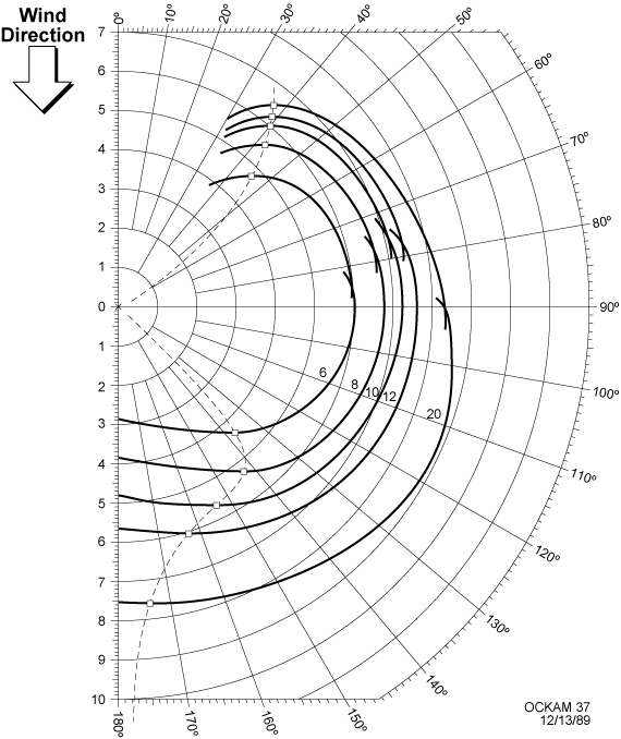
However, for this project, the model captures the fundamental characteristics.
What is Q-learning?
Q-learning is a reinforcement learning algorithm determining the training process to obtain the maximal reward. Given this sailing project example, this is an algorithm for finding the decisions, which will take you as far north as possible. Every time you move north you receive a reward (punishment if you move south). The measure of how well you did is the sum of all the rewards and punishments. \begin{equation} G_t = \sum_{i=t}^T R_i \end{equation} In our case, you can only steer left or right (keeping the steer in place is not possible). So at any time, you want to know in which direction should you steer to receive the biggest return $G_t$. This means that you expect that the selected action will give you $G_t$ reward in the future given your current state. This expectation is called the Q-value. \begin{equation} Q(s_t, a_t) = \mathbb{E}[G_t \mid S = s_t, A = a_t] \end{equation} Where $s_t$ is the state at time $t$ and $a_t$ is the action. But how do we learn this expectation? You may notice that we can expand the $G_t$ term. \begin{align} G_t &= R_t + \sum_{i=t+1}^T R_i \newline G_t &= R_t + G_{t+1} \newline Q(s_t, a_t) &= R_t + Q(s_{t+1}, a_{t+1}) \end{align} In Q-learning we assume that we will always take the best possible action in the future, therefore we can rewrite the equation above to \begin{equation}\label{eq:q_value} Q(s_t, a_t) = R_t + \max_a Q(s_{t+1}, a) \end{equation} Given that this is not immediately satisfied as we don’t know the Q-values beforehand, we will need a learning mechanism. Equation \ref{eq:q_value} resembles a regression task, where we want to decrease the difference between the two sides of the equation. We therefore apply the mean squared error loss function, with the assumption that $\max_a Q(s_{t+1}, a)$ stays constant. As a result we will get the reward prediction error $\delta$ \begin{equation} \delta = R_t + \max_a Q(s_{t+1}, a) - Q(s_t, a_t) \end{equation} which we then apply as an update to the Q-value following the gradient descent strategy using a learning rate $\alpha$. \begin{equation} Q(s_t, a_t) = Q(s_t, a_t) + \alpha \delta \end{equation}
Average Reward
Traditionally Q-learning uses discounting, which means that we decrease the future value by a parameter $\gamma$. The prediction error then becomes \begin{equation} \delta = R_t + \gamma \max_a Q(s_{t+1}, a) - Q(s_t, a_t) \end{equation} This has the effect of applying a smaller value to distant rewards. Here, however, we will use a different approach which uses the average reward. We change the concept of the return such that it will inform us how much above average will the outcome of this action be. \begin{equation} G_t = \sum_{i=t}^T R_i - \rho \end{equation} This results in a slightly altered prediction error. However, it is thought to have a similar or even better effect to discounting. \begin{equation} \delta = R_t - \rho + \max_a Q(s_{t+1}, a) - Q(s_t, a_t) \end{equation} Since we also don’t know the average reward beforehand we will have to learn it. For this purpose we will use moving average. \begin{equation} \rho = \rho + \sigma(R_t - \rho) \end{equation}
Sailing in the open sea
See Demo
The first task that we solve is sailing in the open sea. This means that you are not limited to where you can sail. The goal will be to get as far north as possible. So we will be using the reward function (eq. \ref{eq:reward}) as defined before. There are only two possible actions in this example. Turn slightly left or slightly right. That is also approximately all you can do when steering a sailboat. As the state space, we only use the angle $\theta$, which means that the agent is only allowed to look at the dial of the compass to make decisions.
At the beginning of the article, you saw a simulation of this task. It learned while you run the simulation. This means you had to wait a moment before it began reliably choosing a direction. At first, it was behaving very randomly. However, remember that the agent only knows the angle that the boat is directed and whether it is moving north or not. It first needs to learn what each action means and where the wind is coming from!
As you may have noticed it doesn’t follow a straight line but is rather chaotic. This is because it keeps trying out slightly different routes and the effective outcome doesn’t differ by a lot. So all of them are good routes, although not precisely the best.
Below you can find the python implementation of this simulation.
1
2
3
4
5
6
7
8
9
10
11
12
13
14
15
16
17
18
19
20
21
22
23
24
25
26
27
28
29
30
31
32
33
34
35
36
def angle_to_state(angle):
  return int(30 * ((angle + np.pi) / (2 * np.pi) % 1))  # Discretization of the angle space

def vel(theta, theta_0=0, theta_dead=np.pi/12):
  return 1 - np.exp(-(theta - theta_0)**2 / theta_dead)

def rew(theta, theta_0=0, theta_dead=np.pi/12):
  return vel(theta, theta_0, theta_dead) * np.cos(theta)

Q = np.zeros((30, 2))  # Initialization of the Q-values with zeros
                       # There are 30 angle states and 2 actions

rho = 0  # Initialize the average reward to 0
for episode in range(500):  # run for 500 episodes
  angle = 0  # always start with angle 0
  for i in range(100):
    state = angle_to_state(angle)

    p = np.exp(Q[state]) / np.sum(np.exp(Q[state]))  # Action selection using softmax
    a = np.random.choice(range(2), p=p)  # Sample the action from the softmax distribution

    out = [-0.1, 0.1][a]  # Get the change in angle as a result of the selected angle

    new_state = angle_to_state(angle + out)

    # Calculate the prediction error
    delta = rew(angle + out) - rho + Q[new_state].max() - Q[state, a]

    # Update the average reward
    rho += 0.1 * (rew(angle + out) - rho)

    # Update the Q-value
    Q[state, a] += 0.1 * delta

    # Update the angle
    angle += out
Sailing in a channel
See Demo
The previous example didn’t involve any tacking, however, it was a proof of concept to show that the agent can learn something. Now we will complicate the task for the agent. Let’s introduce two piers on both sides of the reservoir. If the boat swims into a pier it will be destroyed. So now the task is to swim as far north as possible without crashing into the pier.
The piers introduce a terminal condition, which means there will be no actions following the crash. As a result the return from the action leading to the terminal state will give the final reward and there is no prediction following it. \begin{align} G_t &= R_t \newline Q(s_{terminal}, a_t) &= R_t \end{align}
So the prediction error is then simply \begin{align} \delta = R_t \end{align}
Now knowing only about the angle of the boat is not enough. The agent also needs to know how close it is to the pier, so information on the $x$ coordinate is necessary.
It is a more difficult task to the previous one, so learning a good solution will take longer. To help the agent learn faster we will place it at different positions at the beginning of each episode. At first, the agent will crash into the pier all the time, however, after just a couple of episodes, it should start figuring out that maybe a better idea is to tack before hitting the pier. If you simulate long enough you will observe that the agent begins to reliably avoid the piers.
Below you can find the python implementation of this simulation.
1
2
3
4
5
6
7
8
9
10
11
12
13
14
15
16
17
18
19
20
21
22
23
24
25
26
27
28
29
30
31
32
33
34
35
36
37
38
39
40
41
42
43
44
45
46
47
48
49
50
51
52
53
54
55
56
def angle_to_state(angle):
    return int(30 * ((angle + np.pi) / (2 * np.pi) % 1))  # Discretization of the angle space


def x_to_state(x):
    return int(40 * ((x + -10) / 20))  # Discretization of the x space


def vel(theta, theta_0=0, theta_dead=np.pi / 12):
    return 1 - np.exp(-(theta - theta_0) ** 2 / theta_dead)


def rew(theta, theta_0=0, theta_dead=np.pi / 12):
    return vel(theta, theta_0, theta_dead) * np.cos(theta)


Q = np.zeros((30, 40, 2))  # Initialization of the Q-values with zeros
# There are 30 angle states and 2 actions

rho = 0  # Initialize the average reward to 0
for episode in range(500):  # run for 500 episodes
    x = np.random.uniform(-9.9, 9.9)
    angle = 0  # always start with angle 0
    for i in range(100):
        state = angle_to_state(angle)
        x_state = x_to_state(x)

        p = np.exp(Q[state, x_state]) / np.sum(np.exp(Q[state, x_state]))  # Action selection using softmax
        a = np.random.choice(range(2), p=p)  # Sample the action from the softmax distribution

        out = [-0.1, 0.1][a]  # Get the change in angle as a result of the selected angle

        new_state = angle_to_state(angle + out)
        new_x_state = x_to_state(x + vel(angle + out) * np.sin(angle + out))

        # Calculate the prediction error
        if np.abs(x + vel(angle + out) * np.sin(angle + out)) > 10:
            delta = -1  # Terminal case
        else:
            delta = rew(angle + out) - rho + Q[new_state, new_x_state].max() - Q[state, x_state, a]

        # Update the average reward
        rho += 0.1 * (rew(angle + out) - rho)

        # Update the Q-value
        Q[state, a] += 0.1 * delta

        # Update the angle
        angle += out

        # Update the x position
        x += vel(angle + out) * np.sin(angle + out)

        # Stop the episode if the pier was hit
        if np.abs(x) > 10:
            break
Conclusion
We managed to build a simple agent which has learned how to tack to avoid piers. It is a good foundation for further projects, which could involve even more complicated environments. These could have dynamic wind, gusts, obstructions to avoid, weirdly shaped environments, navigating to a certain point. Some further ideas could involve more advanced machine learning techniques since currently the algorithm just uses a tabular representation, which quickly explodes in the number of parameters.
If you found this article helpful, share it with others so that they can also have a chance to find this post. Also, make sure to sign up for the newsletter to be the first to hear about the new articles. If you have any questions make sure to leave a comment or contact me directly.
Want more resources on this topic?
Thanks to Weronika Słowik
Citation
Cite as:
Pierzchlewicz, Paweł A. (Oct 2020). AI learns to sail upwind. Perceptron.blog. https://perceptron.blog/ai-learns-to-sail-upwind/.
Or
@article{pierzchlewicz2020ailearnstosailupwind,
  title   = "AI learns to sail upwind",
  author  = "Pierzchlewicz, Paweł A.",
  journal = "Perceptron.blog",
  year    = "2020",
  month   = "Oct",
  url     = "https://perceptron.blog/ai-learns-to-sail-upwind/"
}