Diffusion models are all the rage these days. They are a new class of generative models, which are capable of generating high-quality images. They have attracted a lot of attention from the machine learning community, as they have been wildly successful in applications such as image generation. They have been especially popular in the task of text-to-image generation, where they have been used to generate images from text descriptions. Some prominent examples include DALL-E 2 by OpenAI, the full-open source StableDiffusion by Stability AI and Midjourney.

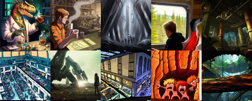
DALL-E 2 generated images to prompts given by me. Example prompt "t-rex mad scientist mixing sparkling substances and drinking tea, digital art".

However, the inner workings of these models can give you quite a headache. They rely on a few concepts and tricks, which might not be obvious at first. In this post, I will lead you through the inner workings of diffusion models on a set of simple toy examples. Ideally, by the of this post, you will have a better understanding and intuition as to how diffusion models work.

You can reproduce the results shown in the post using these colab notebooks.

link	description
	Torch implementation of the Diffusion Model.
	Torch implementation of the Classifier Guided Diffusion.
	Torch implementation of the Classifier-free Guided Diffusion.

Also, the code for this project is available on Github .

Diffusion? What is it?

Diffusion is a process originating from thermodynamics, which describes the process of self-mixing of molecules in a fluid. It is a stochastic process, which is governed by Fick’s law. The diffusion process is a random walk, where the particles move in random directions. The particles are moving in a random direction, but the movement is constrained by the diffusion coefficient. As defined by Fick’s law, the particles will move from a region of high concentration to a region of low concentration. This coefficient determines the speed of the particles. \begin{equation*} J = -D \nabla_x C \end{equation*} where $J$ is the flux of the particles, $D$ is the diffusion coefficient and $C$ is the concentration of the particles in space $x$. A popular example of diffusion is the mixing of tea in a cup of water. The particles of tea are moving from the region of high concentration (the tea bag) to the region of low concentration (the water). Effectively, after a while, the particles will be uniformly distributed in the water and you will get a cup of tea.

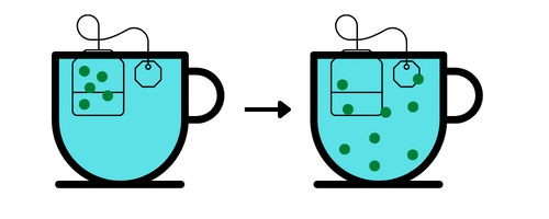
Diffusion of tea particles in water.

Diffusion Models

(Sohl-Dickstein et al., 2015) introduced the concept of diffusion models to the machine learning community in 2015. They define a forward diffusion process the process of gradually adding noise to the input data until it becomes just noise. They then propose to learn the reverse diffusion process - the process of gradually removing noise from the data until it becomes the original data. (Ho et al., 2020) showed that this process can be used to generate high-quality images.

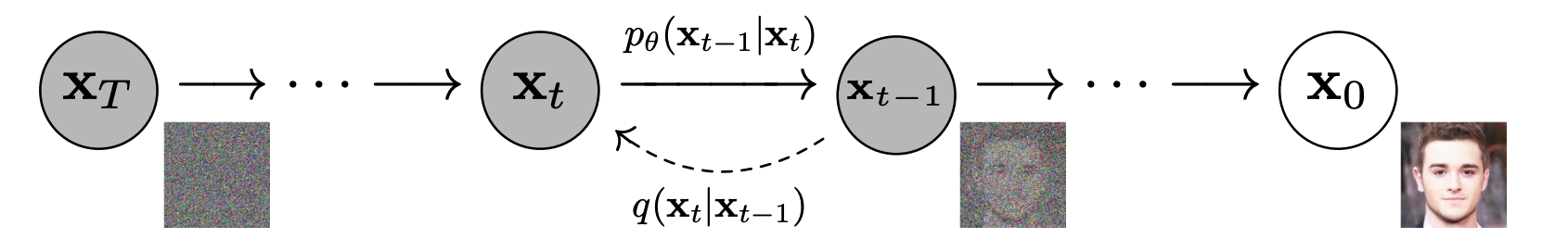
Graphical model of a diffusion model (Ho et al., 2020). Forward process from image to noise and reverse process from noise to image.

In the next sections we will examine in-depth how both the forward and reverse diffusion processes work. I also refer you to (Weng, 2021) which is a great post that explains the diffusion process and provided a lot of intuition for me.

Forward Diffusion Process

We are given a sample $\vx_0$ from the data distribution $q(\vx)$. The forward diffusion process gradually adds Gaussian noise with variance $\beta_t$ to the sample $\vx_t$ at time $t$ over $T$ steps (Sohl-Dickstein et al., 2015). A single step can be defined as \begin{equation}\label{eq:forward_step} \vx_{t} = \sqrt{1 - \beta_t} \vx_{t-1} + \sqrt{\beta_t} \vepsilon_{t-1} \end{equation} where $\vepsilon_t$ is a sample from a standard Gaussian distribution $\mathcal{N}(\vepsilon_t; \mathbf{0}, \mathbf{I})$. As a result, the more steps we take, the more noise we add to the sample and the less of the original features are left. The added noise can be defined as a transition probability of a Markov Process. \begin{equation*} q(\vx_t \mid \vx_{t-1}) = \mathcal{N}(\vx_t; \sqrt{1 - \beta_t}\vx_{t-1}, \beta_t\mathbf{I}) \end{equation*} The set of all states $\mathcal{T} = {\vx_0, \vx_1, \dots, \vx_T}$ is called the diffusion trajectory. Since it is a Markov process, the current state only depends on the previous state. So we can define the probability of the entire trajectory $\mathcal{T}$ as \begin{equation*} q(\vx_{1:T} \mid \vx_0) = \prod_{t=1}^T q(\vx_t \mid \vx_{t-1}) \end{equation*} We can simulate the forward diffusion process for a set of simple 2D datasets and visualize the trajectories of the samples. As we can see, the samples at the beginning retain the original features of the dataset, but as we add more noise, the samples resemble more and more the standard Gaussian distribution.

Forward diffusion process. Three examples of the forward diffusion process applied on different datasets. I. Swiss Roll, II. Moons and III. Mixture of Gaussians.

1
2
3
4
5
6
7
8
9
10
11
12
13
14
import torch
import numpy as np
from sklearn.datasets import make_moons, make_swiss_roll

x_0, c = make_swiss_roll(100, noise=0.1)
x_0 = torch.Tensor(x_0[:, [0, 2]])
x_0 = (x_0 - x_0.mean()) / x_0.std()

beta = 0.01
T = 50

x = x_0.clone()
for i in range(T):
    x = x * np.sqrt(1 - beta) + np.sqrt(beta) * torch.randn(len(x_0), 2)

Deriving the forward diffusion process

As we saw the forward diffusion process works, however, where does equation $\eqref{eq:forward_step}$ come from? As I have shown in a previous blog post on Langevin Dynamics a stochastic process with the steady state distribution $p(\vx)$ (also known as Langevin Diffusion) is defined as \begin{equation}\label{eq:langevin_diffusion} \vx_{t} = \vx_{t-1} + \nabla_{\vx} \log p(\vx_{t-1}) \vepsilon + \sqrt{2 \vepsilon}\ \vz \end{equation} where $\vz \sim \mathcal{N}(\mathbf{0}, \mathbf{I})$. The gradient $\nabla_{\vx} \log p(\vx_{t-1})$ (score function) for a Standard Gaussian distribution is $-\vx_{t-1}$, thus we can rewrite equation $\eqref{eq:langevin_diffusion}$ as \begin{align*} \vx_{t} &= \vx_{t-1} - \vx_{t-1} \vepsilon + \sqrt{2 \vepsilon}\ \vz\newline &= (1 - \vepsilon) \vx_{t-1} + \sqrt{2 \vepsilon}\ \vz \end{align*} Next we need to define the variance of the noise $\vepsilon$. We substitute the $\beta = 2\vepsilon$. \begin{align}\label{eq:langevin_before_taylor} \vx_{t} &= \left(1 - \frac{1}{2} \beta\right) \vx_{t-1} + \sqrt{\beta}\ \vz \end{align} Then we observe that $1 - \frac{1}{2} \beta$ are the first two terms of the Taylor expansion of $\sqrt{1 - \beta}$ at $0$. Thus, we can rewrite equation $\eqref{eq:langevin_before_taylor}$ as \begin{align*} \vx_{t} &= \sqrt{1 - \beta} \vx_{t-1} + \sqrt{\beta}\ \vz \end{align*} which is exactly equation $\eqref{eq:forward_step}$ for the forward diffusion process.

Reparametrization trick to sample $x_t$ at arbitrary time $t$

Under equation $\eqref{eq:forward_step}$ obtaining the sample $\vx_t$ at time $t$ is costly, as we need to perform $t$ steps of the forward diffusion process. It is possible to sample $\vx_t$ at arbitrary time $t$ by using the reparametrization trick. By substituting $\alpha_t = 1 - \beta_t$ we can rewrite the update step in equation $\eqref{eq:forward_step}$ as \begin{equation*} \vx_{t} = \sqrt{\alpha_t} \vx_{t-1} + \sqrt{1 - \alpha_t} \vepsilon_{t-1} \end{equation*} We can unfold the update step to define $\vx_{t}$ in terms of $\vx_{t-2}$ by recursively substituting $\vx_{t-1}$. \begin{align*} \vx_{t} &= \sqrt{\color{violet}{\alpha_{t}}} \color{orange}{\vx_{t-1}} + \sqrt{1 - \alpha_t} \vepsilon_{t-1}\newline &= \sqrt{\color{violet}{\alpha_{t}}} \color{orange}{\left(\sqrt{\alpha_{t-1}} \vx_{t-2} + \sqrt{1 - \alpha_{t-1}} \vepsilon_{t-2}\right)} + \sqrt{1 - \alpha_t} \vepsilon_{t-1}\newline &= \sqrt{\color{violet}{\alpha_{t}}\alpha_{t-1}} \vx_{t-2} + \underbrace{\sqrt{\color{violet}{\alpha_{t}}(1 - \alpha_{t-1})} \vepsilon_{t-2}}_{\mathcal{N}(\vepsilon_{t-2};\ \mathbf{0},\ \alpha_{t}(1 - \alpha_{t-1}) \mathbf{I})} + \underbrace{\sqrt{1 - \alpha_t} \vepsilon_{t-1}}_{\mathcal{N}(\vepsilon_{t-1};\ \mathbf{0},\ (1 - \alpha_{t}) \mathbf{I})}\newline \end{align*} The second and third terms are simply a sum of two independent Gaussian distributions. You may recall that the variance of a sum of independent Gaussian distributions is simply $\sigma^2_{1+2} = \sigma_1^2 + \sigma_2^2$. So here the summed variance is \begin{equation*} \sigma^2 = \sigma_{t}^2 + \sigma_{t-1}^2 = (1 - \alpha_{t}) + \alpha_{t} (1 - \alpha_{t-1}) = 1 - \alpha_{t} \alpha_{t-1} \end{equation*} Thus we can rewrite the update step as \begin{equation*} \vx_t = \sqrt{\alpha_{t}\alpha_{t-1}} \vx_{t-2} + \sqrt{1 - \alpha_t\alpha_{t-1}} \vepsilon_{t-2} \end{equation*} Analogously we can keep on recursively unfolding the update step until we reach $\vx_0$. A pattern emerges allowing a nice property to be derived. If we substite $\bar{\alpha}_t = \prod_{i=1}^{t} \alpha_{i}$ the state $\vx_t$ can be written as \begin{equation*} \vx_{t} = \sqrt{\bar{\alpha_{t}}} \vx_{0} + \sqrt{1 - \bar{\alpha_t}} \vepsilon_{0} \end{equation*} allowing us to compute the variance of the state at time $t$ directly, without having to iterate over the entire trajectory.

$\bar{\alpha}_t$ as a signal-to-noise ratio

The variable $\bar{\alpha}_t$ indicates the amount of the original signal that is left in the state $\vx_t$. That is at time $0$ the state $\vx_0$ is the original data point and $\bar{\alpha}_0 = 1$. As time progresses more noise is added and the original data point becomes diluted. By the end of the trajectory $\bar{\alpha}_T = 0$ and the state $\vx_T$ is simply noise.

Reverse Diffusion Process

The forward diffusion process is well-defined and we can easily sample from it. However, we are actually interested in the reverse diffusion process. If we could reverse the added noise at $\vx_t$ we would be able to generate samples from the data distribution, using only samples from the standard Gaussian distribution. For this to be possible we would need to be able to evaluate $q(\vx_{t-1} \mid \vx_t)$. Unfortunately, $q(\vx_{t-1} \mid \vx_t)$ is not tractable, but we do know a few things about it.

Gaussian Form of the Reverse Diffusion Process

To build the inverse diffusion process we need to invert $q(\vx_{t} \mid \vx_{t-1})$ which is a Gaussian distribution. (Feller, 1949) show that for very small variance $\beta \rightarrow 0$ the reverse density $q(\vx_{t-1} \mid \vx_t)$ will also be Gaussian. Essentially, this imposes the requirement that the size of the change needs to be small enough that the change in the distribution is almost negligible. However, across the entire trajectory the small changes pile up and together will result in a non-negligible effect. The plot below shows a schematic of the forward and reverse diffusion processes and the associated distributions.

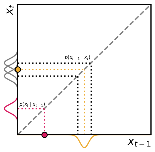
Schematic of the forward and reverse probability distributions for a Gaussian distribution. Forward (pink) shows that given the observation $\vx_t$ the distribution of $\vx_{t-1}$ is a Gaussian distribution. The reverse (orange) shows that given the observation $\vx_{t-1}$ the distribution of $\vx_t$ is also a Gaussian distribution.

Oracle reverse diffusion process

Even though $q(\vx_{t-1} \mid \vx_t)$ is not tractable, (Ho et al., 2020) identified that in the case where $\vx_0$ is known it is possible condition on $\vx_0$ to obtain a tractable distribution. \begin{equation*} q(\vx_{t-1} \mid \vx_t, \vx_0) = \mathcal{N}\left(\vx_{t-1}; \tilde{\mu}_\theta(\vx_t, \vx_0), \tilde{\beta}_t\mathbf{I}\right) \end{equation*} Then using the Bayes’ rule we have \begin{equation*} q(\vx_{t-1} \mid \vx_t, \vx_0) = q(\vx_t \mid \vx_{t-1}, \vx_0)\frac{q(\vx_{t-1} \mid \vx_0)}{q(\vx_t \mid \vx_0)} \end{equation*} Thanks to the Markov property we can rewrite this as \begin{equation*} q(\vx_{t-1} \mid \vx_t, \vx_0) = \color{red}{q(\vx_t \mid \vx_{t-1})}\frac{\color{violet}{q(\vx_{t-1} \mid \vx_0)}}{\color{orange}{q(\vx_t \mid \vx_0)}} \end{equation*} As we now know each of these expressions we can write that \begin{equation*} q(\vx_{t-1} \mid \vx_t, \vx_0) \propto \exp\left(- \frac{1}{2}\left( \color{red}{\frac{(\vx_t - \sqrt{\alpha_t}\vx_{t-1})^2 }{1 - \alpha_t}} + \color{violet}{\frac{(\vx_{t-1} - \sqrt{\bar{\alpha}_{t-1}}\vx_0)^2}{1 - \bar{\alpha}_{t-1}}} - \color{orange}{\frac{(\vx_{t} - \sqrt{\bar{\alpha_t}}\vx_0)^2}{1 - \bar{\alpha_t}}} \right) \right) \end{equation*} (Weng, 2021) does a really nice job deriving the final expression for the mean and variance of the reverse diffusion process. The mean is given by \begin{equation*} \tilde{\mu}_t = \frac{1}{\sqrt{\alpha_t}}\left(\vx_t - \frac{1 - \alpha_t}{\sqrt{1 - \bar{\alpha_t}}} \vepsilon_t \right) \end{equation*} and the variance is \begin{equation*} \tilde{\beta}_t = \frac{1 - \bar{\alpha}_{t-1}}{1 - \bar{\alpha_t}} \beta_t \end{equation*} Note that the mean and variance are not functions of $\vx_0$! However, this assumes that we know $\vx_0$ before we start the reverse diffusion process and that $\vx_t$ comes from the known $\vx_0$. The benefit is that at training time we can compute the ideal mean and variance to obtain $\vx_0$ and then train a neural network to learn an approximate distribution $p_\theta(\vx_{t-1} \mid \vx_t)$ of the oracle distribution $q(\vx_{t-1} \mid \vx_t)$.

Oracle reverse diffusion process. You can reverse the diffusion if you know $\vx_0$.

Training a Diffusion Model

Now that we have an understanding of the forward and reverse diffusion processes we can start training a diffusion model. In fact it is very similar to training a VAE. We can simply compute the evidence lower bound (ELBO) as \begin{align*} \log p(\vx) &\leq \mathbb{E}_{q(\vx_{0:T})}\left[\log \frac{q(\vx_{1:T} \mid \vx_0)}{p_\theta(\vx_{0:T})} \right] \newline &= \mathbb{E}_{q}{\Large{[}}\underbrace{KL(q(\vx_T \mid \vx_0) : p(\vx_T))}_{L_T} \newline &+ \sum_{t=2}^T \underbrace{KL(q(\vx_{t-1} \mid \vx_t, \vx_0) : p_\theta(\vx_{t-1} \mid \vx_t))}_{L_{t-1}} \newline &- \underbrace{\log p_\theta(\vx_0 \mid \vx_1)}_{L_0}{\Large{]}}\newline &= L_T + \sum_{t=2}^T L_{t-1} - L_0 \end{align*}

• $L_T$ is the KL divergence between the posterior distribution $q(\vx_T \mid \vx_0)$ and the prior distribution $p(\vx_T)$. It compares whether $q(\vx_T \mid \vx_0)$ is a standard Gaussian distribution and thus is a constant.
• $L_0$ is a reconstruction term, verifying whether the original $\vx_0$ can be reconstructed. (Ho et al., 2020) use a separate discrete decoder for this term.
• $\sum_{t=2}^T L_{t-1}$ also denoted as $L_{t}$ formulates the difference between the desired denoising step and the predicted denoising step. Thus, the core objective of the diffusion model is $L_{t}$.

We define the approximate reverse diffusion process as \begin{equation*} p_\theta(\vx_{t-1} \mid \vx_t) = \mathcal{N}\left(\vx_{t-1}; \tilde{\mu}_\theta(\vx_t, t), \tilde{\beta}_t\mathbf{I}\right) \end{equation*} As per the loss function we would like $\mu_{\theta}(\vx_t, t)$ to predict $\tilde{\mu}_t$. Since $\vx_t$ is available as input and $\alpha_t$ is known we can reparametrize the Gaussian noise to be predicted. \begin{equation*} \mu_{\theta}(\vx_t, t) = \frac{1}{\sqrt{\alpha_t}}\left(\vx_t - \frac{1 - \alpha_t}{\sqrt{1 - \bar{\alpha_t}}} \vepsilon_\theta(\vx_t, t) \right) \end{equation*} The loss function is then given by the difference between the predicted and the desired mean. \begin{align*} L_{t} &= \mathbb{E}_{\vx_0, \vepsilon}\left[\frac{1}{2||\Sigma_\theta(\vx_t, t)||^2_2}\left|\left|\color{violet}{\mu_{\theta}(\vx_t, t)} - \color{orange}{\tilde{\mu}_t(\vx_t, \vx_0)}\right|\right|^2\right]\newline &= \mathbb{E}_{\vx_0, \vepsilon}{\Large{[}}\frac{1}{2||\Sigma_\theta(\vx_t, t)||^2_2}{\Large{||}}\color{violet}{\frac{1}{\sqrt{\alpha_t}}\left(\vx_t - \frac{1 - \alpha_t}{\sqrt{1 - \bar{\alpha_t}}} \vepsilon_\theta(\vx_t, t) \right)} - \color{orange}{\frac{1}{\sqrt{\alpha_t}}\left(\vx_t - \frac{1 - \alpha_t}{\sqrt{1 - \bar{\alpha_t}}} \vepsilon_t \right)}{\Large{||}}^2{\Large{]}}\newline &= \mathbb{E}_{\vx_0, \vepsilon}\left[\frac{(1 - \alpha_t)^2}{2\alpha_t(1 - \bar{\alpha}_t)||\Sigma_\theta(\vx_t, t)||^2_2}\left|\left|\vepsilon_t - \vepsilon_\theta\left(\vx_t, t\right)\right|\right|^2\right]\newline &= \mathbb{E}_{\vx_0, \vepsilon}\left[\frac{(1 - \alpha_t)^2}{2\alpha_t(1 - \bar{\alpha}_t)||\Sigma_\theta(\vx_t, t)||^2_2}\left|\left|\vepsilon_t - \vepsilon_\theta\left(\sqrt{\bar{\alpha}_t} \vx_0 + \sqrt{1 - \bar{\alpha}_t}\vepsilon_t, t\right)\right|\right|^2\right] \end{align*}

Simplifying the Loss Function

(Ho et al., 2020) found that better results can be achieved by simplifying the loss function. In particular, they find that dropping the weight term improves sample quality. Hence, a simplified term is used \begin{align*} L_t^{simple} &= \mathbb{E}_{t\sim\mathcal{U}[1,T], \vx_0, \vepsilon}\left[\left|\left|\vepsilon_t - \vepsilon_\theta\left(\vx_t, t\right)\right|\right|^2\right]\newline &= \mathbb{E}_{t\sim\mathcal{U}[1,T], \vx_0, \vepsilon}\left[\left|\left|\vepsilon_t - \vepsilon_\theta\left(\sqrt{\bar{\alpha}_t} \vx_0 + \sqrt{1 - \bar{\alpha}_t}\vepsilon_t, t\right)\right|\right|^2\right] \end{align*}

Sampling of $t$ from the uniform distribution. Thus the training essentially boils down to minimizing the MSE between the oracle reverse diffusion noise and the predicted reverse diffusion noise.

Link to denoising score matching

Essentially, the diffusion model is trained on a denoising score matching objective (Vincent, 2011), between the inverse diffusion process and the oracle diffusion process. Consider pairs of clean and corrupted examples $(\vx, \tilde{\vx})$. For the joint distribution $p(\vx, \tilde{\vx})$ we can define the denoising score as \begin{equation*} \mathcal{S}(\vx, \tilde{\vx}) = \mathbb{E}_{q}\left[\left|\left| \psi(\tilde{\vx}, \theta) - \frac{\partial \log q(\tilde{\vx} \mid \vx)}{\partial \tilde{\vx}} \right|\right|^2\right] \end{equation*} where $\psi(\tilde{\vx}, \theta)$ is the score of $q(\tilde{\vx}; \theta)$. For the Gaussian distribution $q$ we have \begin{equation*} \frac{\partial \log q(\tilde{\vx} \mid \vx)}{\partial \tilde{\vx}} = \frac{1}{\sigma^2}(\tilde{\vx} - \vx) \end{equation*} Consider our diffusion process where we corrupt a sample $x$ with Gaussian noise $\vepsilon$ with variance $\sigma^2$. Thus by substituting our assumptions we find the above expression is proportional to $\vepsilon_t$.

\begin{align*} \frac{1}{\sigma^2}(\tilde{\vx} - \vx) &= \frac{1}{\sigma^2}(\sqrt{1 - \beta_t} \vx + \sqrt{\beta_t} \vepsilon_t - \vx)\newline &= \frac{1}{\sigma^2}(\vx \underbrace{(1 - \sqrt{1 - \beta_t})}_{\approx 0} + \sqrt{\beta_t} \vepsilon_t)\newline &\approx \frac{1}{\beta_t}(\sqrt{\beta_t} \vepsilon_t )\newline &\propto \vepsilon_t\newline \end{align*}

Thus the denoising score is \begin{equation*} \mathcal{S}(\vx, \tilde{\vx}) = \mathbb{E}_{q}\left[\left|\left| \psi(\tilde{\vx}, \theta) - \vepsilon_t \right|\right|^2\right] \end{equation*} which resembles the loss function used in the training of the diffusion model. Thus, this indicates that the network $\vepsilon_\theta$ should learn the score function $\psi$ of the target distribution.

Implementation

Model Architecture

For the toy problem we explore a simple architecture with three layers $3 \rightarrow 100$, $100 \rightarrow 100$, $100 \rightarrow 3$ dimension and ReLU activation.

1
2
3
4
5
6
7
8
9
10
11
12
13
14
15
16
17
18
19
20
21
import torch.nn as nn
import torch

class DiffusionModel(nn.Module):
  def __init__(self):
    super().__init__()
    
    self.layers = nn.Sequential(
      nn.Linear(3, 100),
      nn.ReLU(),
      nn.Linear(100, 100),
      nn.ReLU(),
      nn.Linear(100, 3)
    )

  def position_embedding(self, x_t, t):
    return torch.cat([x_t, t.repeat(x_t.shape[0], 1)], dim=1)

  def forward(self, x_t, t):
    inp = self.position_embedding(x_t, t)
    return self.layers(inp)

Training

(Ho et al., 2020) devise a training procedure that allows us to easily train the diffusion model.

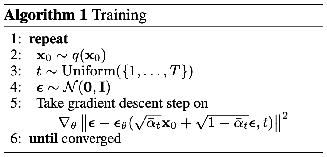
Algorithm for training the diffusion model. (Ho et al., 2020)

The training procedure is as follows:

1. Take a data sample $\vx_0$ from the target distribution $q(\vx_0)$.
2. Sample a time $t$ from the uniform distribution $\mathcal{U}[1,T]$.
3. Sample a noise vector $\vepsilon$ from the standard normal distribution $\mathcal{N}(\mathbf{0}, \mathbf{I})$.
4. Compute the corrupted sample $\tilde{\vx} = \sqrt{\bar{\alpha}_t} \vx_0 + \sqrt{1 - \bar{\alpha}_t} \vepsilon$ at time $t$.
5. Compute the error between the oracle diffusion noise $\vepsilon_t$ and the predicted diffusion noise $\vepsilon_\theta(\tilde{\vx}, t)$.
6. Take a gradient step on the loss function.

1
2
3
4
5
6
7
8
9
10
11
12
13
14
15
16
17
18
19
20
21
22
23
24
25
26
27
28
29
30
import torch
from tqdm import tqdm

# Training parameters
beta = 0.01
alpha = 1 - beta
T = 20
EPOCHS = 10_000
bs = x_0.shape[0] # batch size

# Training loop
model = DiffusionModel()
optimizer = torch.optim.Adam(model.parameters())

for i in range(EPOCHS):
  optimizer.zero_grad()

  t = torch.randint(0, T, size=(1, )) # sample t from uniform distribution
  alpha_bar = alpha**(T - t)
  eps_true = torch.randn(bs, 2) # sample noise from standard normal distribution
  
  # corrupt x_0 with noise
  corrupted_x = torch.sqrt(alpha_bar) * x_0 + torch.sqrt(1 - alpha_bar) * eps_true

  eps_pred = model(corrupted_x, t) # predict noise at time t

  loss = mse(eps_true, eps_pred) # compute MSE loss
  loss.backward()

  optimizer.step()

We can visualize the MSELoss over the training steps. It is important to observe, that the loss is very noisy and it may be difficult to determine whether the model is still improving.

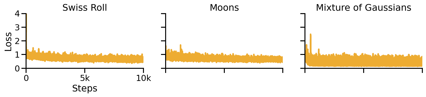
Training loss for the three toy problems. The loss is very noisy and it may be difficult to determine whether the model is still improving.

Sampling

With the trained diffusion model we can now generate samples from the target distribution.

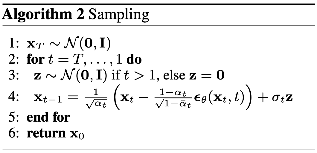
Algorithm for sampling from the diffusion model. (Ho et al., 2020)

The sampling procedure is as follows:

1. Sample $\vx_T$ from a standard normal distribution $\mathcal{N}(0, I)$.
2. Iterate over $t$ from $T$ to $1$:
   1. Sample a noise vector $\vz$ from a standard normal distribution $\mathcal{N}(0, I)$.
   2. Compute the diffusion noise $\vepsilon_\theta(\vx_t, t)$.
   3. Compute the denoising step using Langevin dynamics.

1
2
3
4
5
6
7
8
9
10
import torch
import numpy as np
x_t = torch.randn(200, 2)

for t in range(1, 30):
    z = torch.randn(x_t.shape[0], 2)
    
    with torch.no_grad():
        eps = model(x_t, torch.Tensor([t]))
        x_t = 1/np.sqrt(alpha) * (x_t - (1 - alpha)/np.sqrt(1 - alpha**t)) * eps) + beta * z

We can visualize the denoising process by plotting the denoised samples at each time step.

Sampling from a trained diffusion model. I parametrized the model to be able to sample past the training $T$ (I used 30 timesteps for sampling instead of 20). I find that these addional few steps greatly improve the sample quality.

With the trained model we can also inspect $\vepsilon_\theta$. According to the connection to denoising score matching, we expect $\vepsilon_\theta$ to learn the score function $\psi$ of the target distribution. Thus, we visualize the output of $\vepsilon_\theta$ as a gradient map. We can indeed see that $\vepsilon_\theta$ corresponds to the score function of the target distribution.

Actual output of the network $\vepsilon_\theta$. As can be visible it corresponds to the gradient field of the log probability density function.

Some engineering tricks

The above implementation is built to be as simple as possible. However, there are a few additional tricks that can be used to improve the performance of the model.

Positional Embeddings

Here we used an identity embedding for the time $t$, meaning that the model took time $t$ as a direct input. However, (Ho et al., 2020) used a sinsoidal position embedding inspired by the Transformer (Vaswani et al., 2017). This positional embedding is a function of the time $t$ and the dimension $d$ of the input. The positional embedding is defined as follows: \begin{align*} \text{PE}(t, 2i) &= \sin(t / 10000^{2i / d}) \newline \text{PE}(t, 2i + 1) &= \cos(t / 10000^{2i / d}) \end{align*} Each dimension of the embedding is a sinusoid of a different frequency ranging from $2\pi$ to $10000\cdot 2\pi$. The positonal embedding is added to the input of the network.

1
2
3
4
5
6
7
8
9
10
11
def position_embedding(self, x, t):
    """
    Computes the position embedding for the input x.
    """
    d = x.shape[-1]
    t = t / 10000 ** (torch.arange(0, d, 2) / d)
    t = torch.stack((torch.sin(t), torch.cos(t)), dim=1).reshape(d)
    return torch.cat([x, t.repeat(x.shape[0], 1)], dim=1)
    
# Add the new position embedding to the DiffusionModel class
DiffusionModel.position_embedding = position_embedding

Variance Scheduling

We kept the variance $\beta_t$ constant throughout the training. However, (Ho et al., 2020) used variance scheduling. The simplest form of variance scheduling is to linearly increase the variance from $\beta_1$ to $\beta_T$ over the training steps. (Ho et al., 2020) scaled the variance $\beta$ from $\beta_1 = 10^-4$ to $\beta_T = 0.02$ for image pixel values in the range [-1, 1].

1
2
3
4
5
def linear_variance_scheduling(T, beta_1=1e-4, beta_T=0.02):
    """
    Precomputes the variance for each time step.
    """
    return beta_1 + (beta_T - beta_1) * np.arange(T) / (T - 1)

(Nichol & Dhariwal, 2021) found that variance scheduling can be improved by using a cosine schedule for low resolution images. They identified that towards the end sample is too noisy and so it does not contribute much to the sample quality.

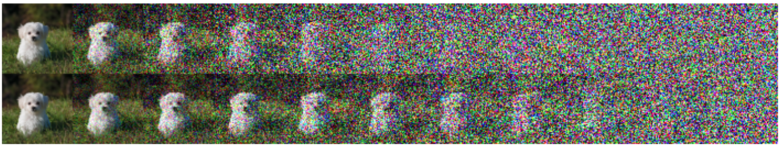
Comparison of the noisyness of images under different variance schedules. Top is linear, bottom is cosine. (Nichol & Dhariwal, 2021)

In fact, (Nichol & Dhariwal, 2021) observed that in the case of the linear scheduling 20% of initial steps in the reverse process could be skipped without influencing the quality of samples. They define the cosine schedule as follows: \begin{align*} \beta(t) &= 1 - \frac{\bar{\alpha}_t}{\bar{\alpha}_{t-1}} \newline \bar{\alpha}_t &= \frac{f(t)}{f(0)} \newline f(t) &= \cos\left(\frac{\pi}{2} \cdot \frac{t/T + s}{1 + s}\right)^2 \end{align*} where $s$ is a small offset. In practice, they also clip $\beta$ to be no larger than $0.999$ to avoid singuilarities at the end of the diffusion.

1
2
3
4
5
6
7
def cosine_variance_scheduling(T, s=1e-6, beta_max=0.999):
    """
    Precomputes the variance for each time step.
    """
    f = lambda t: torch.cos((np.pi/2) * (t/T + s) / (1 + s))**2
    alpha = f(torch.arange(T)) / f(0)
    return torch.clamp(1 - alpha[1:] / alpha[:-1], max=beta_max)

We can compare the different schedules by visualizing the variance $\beta_t$ and $\bar{\alpha}_t$. Based on these plots we can see that the original signal drops of the fastest in the constant variance schedule whereas, in the cosine schedule, some part of the signal is preserved almost until the end.

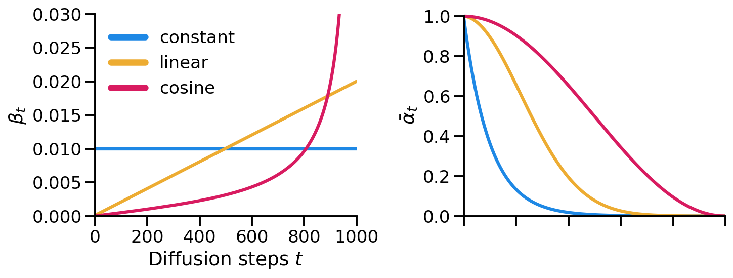
Comparison of different variance schedules.

Conditional Diffusion Models

A powerful use-case of diffusion models is to use them for conditional generation. In this section we will look at how to use diffusion models for conditional generation.

Guided Diffusion

We can add conditioning information $y$ at every step of the diffusion process. \begin{equation*} p_\theta(\vx_{0:T} \mid \vy) = p_\theta(\vx_T) \prod_{t=1}^T p_\theta(\vx_t \mid \vx_{t-1}, \vy) \end{equation*} In general, guided diffusion models aim to learn $\nabla \log p_\theta(\vx_t \mid \vy)$ (missing reference). Using Bayes’ rule we can rewrite the above equation as follows: \begin{align*} \nabla_{\vx_t} \log p_\theta(\vx_t \mid \vy) &= \nabla_{\vx_t} \log \frac{p_\theta(\vy \mid \vx_{t}) p_\theta{\vx_t}}{p_\theta(\vy)} \newline &= \nabla_{\vx_t} \log p_\theta(\vy \mid \vx_{t}) + \nabla_{\vx_t} \log p_\theta(\vx_t) - \underbrace{\nabla_{\vx_t} \log p_\theta(\vy)}_{=0} \newline &= \nabla_{\vx_t} \log p_\theta(\vy \mid \vx_{t}) + \nabla_{\vx_t} \log p_\theta(\vx_t) \end{align*} A guidance scalar term $s$ is also added. \begin{equation*} \nabla_{\vx_t} \log p_\theta(\vx_t \mid \vy) = s \cdot \nabla_{\vx_t} \log p_\theta(\vy \mid \vx_{t}) + \nabla_{\vx_t} \log p_\theta(\vx_t) \end{equation*} With this parametrization we can distinguish two types of guided diffusion models: classifer guidance and classifier-free guidance.

Classifier Guidance

(Dhariwal & Nichol, 2021) trained a classifier $f_\phi(\vy \mid \vx_t)$ on noisy data $\vx_t$ and used the gradients $\nabla_{\vx_t} \log f_\phi(\vy \mid \vx_t)$ to guide the diffusion. Thus the score function of the joint distribution is: \begin{align*} \nabla_{\vx_t} \log q_\theta(\vx_t, \vy) &= \nabla_{\vx_t} \log q(\vx_t) + s\nabla_{\vx_t} \log q(\vy \mid \vx_t)\newline &\approx -\frac{1}{\sqrt{1 - \bar{\alpha}_t}} \vepsilon_\theta(\vx_t, t) + s\nabla_{\vx_t} \log f_\phi(\vy \mid \vx_t)\newline &= -\frac{1}{\sqrt{1 - \bar{\alpha}_t}} \left(\vepsilon_\theta(\vx_t, t) - s\sqrt{1 - \bar{\alpha}_t}\nabla_{\vx_t} \log f_\phi(\vy \mid \vx_t)\right) \end{align*} Thus the classifier-guided predictor is defined as follows: \begin{equation*} \vepsilon_\theta(\vx_t, t) = \vepsilon_\theta(\vx_t, t) - s\sqrt{1 - \bar{\alpha}_t}\nabla_{\vx_t} \log f_\phi(\vy \mid \vx_t) \end{equation*}

We can test this approach on the 2D toy problem. I trained a classifier with 1 full-connected hidden layer with 100 neurons and ReLU activation.

1
2
3
4
5
6
7
8
9
10
11
12
13
14
15
16
import torch.nn as nn
import torch.nn.functional as F

class Classifier(nn.Module):
    def __init__(self):
        super().__init__()
        self.layers = nn.Sequential(
            nn.Linear(3, 100),
            nn.ReLU(),
            nn.Linear(100, 2)
        )

    def forward(self, x, t):
        inp = torch.cat([x, t.repeat(x.shape[0]).unsqueeze(1)], dim=1)
        logits = self.layers(inp)
        return logits

It was trained to predict the class $y$ of the data point $\vx_t$ at each timestep $t$ of the diffusion process. The code, learning curve and a simulation with classification is shown below.

1
2
3
4
5
6
7
8
9
10
11
12
13
14
15
16
17
18
19
20
21
22
23
24
25
26
27
28
EPOCHS = 500

beta = 0.01
alpha = 1 - beta
T = 20

clf = Classifier()
optimizer = torch.optim.Adam(clf.parameters())

for i in range(EPOCHS):
  optimizer.zero_grad()

  bs = x_0.shape[0]
  t = torch.randint(0, T, size=(1, ))
  alpha_bar = alpha**(T - t)
  eps = torch.randn(bs, 2)

  corrupted_x = torch.sqrt(alpha_bar) * x_0 + torch.sqrt(1 - alpha_bar) * eps

  logits = clf(corrupted_x, t)

  # One-hot encode the labels
  y_true = F.one_hot(torch.LongTensor(labels), 2).float()
  
  loss = F.cross_entropy(logits, y_true)
  loss.backward()

  optimizer.step()

Learning curve of the classifier and predicted classes across diffusion steps.

With the trained classifier we are able to guide the diffusion process using the gradients of the classifier. However, let’s first look at the gradients of the classifier and see if they provide any useful insight.

The gradient with respect to $\vx_t$ of the classifier for class 0 and class 1.

1
2
3
4
5
6
7
8
9
10
11
12
13
14
15
16
17
18
19
20
21
22
def classifier_grad(clf, x, y, s=1):
  """
  Compute the gradient of the classifier with respect to x.
  params:
    clf: classifier
    x: input
    y: label of the class to compute the gradient for
    s: gradient importance weight
  """
  x_in = x.detach().requires_grad_(True)

  logits = clf(x_in, torch.Tensor([t]))
  log_probs = F.log_softmax(logits, dim=-1)

  # Select the log probabilities of the class y
  log_probs = log_probs[range(len(logits)), torch.LongTensor([y]).view(-1)]
  log_probs = log_probs.sum()
  
  # Compute the gradient of the log probabilities with respect to x
  grad = torch.autograd.grad(log_probs, x_in)[0]
  
  return grad * s

What we can see is that in this simple case the gradients will push the points out of the other classes region. Now let’s see how the guided diffusion performs.

Classifier-guided diffusion process generating data points from either class 0 or class 1.

1
2
grad_0 = classifier_grad(cls, x_0, y=0, s=3)
eps_0 = mog_net(x_0, torch.Tensor([t])).detach() - np.sqrt(1 - alpha**t) * grad_0

Success! We managed to guide the diffusion process to generate points from a specific class. Let’s look also at the output of the score functions for generating these two classes.

Score functions for generating data points from either class 0 or class 1.

As we can see the score functions for each of the classes correspond to a score function for generating a Gaussian distribution with the same mean and variance as the class.

Classifier-free Guidance

(Ho & Salimans, 2022) propose a classifier-free approach to guide the diffusion process. Instead of training a separate classifier, they used a conditional diffusion model $\vepsilon_\theta(\vx_t \mid \vy)$ with an unconditional diffusion model $\vepsilon_\theta(\vx_t)$. The authors used the exact same network to model both the conditional and unconditional noise. To achieve this during training they randomly set the conditioning vector $y$ to 0. The score function $\nabla_{\vx_t} \log p(\vy \mid \vx_t)$ is defined as: \begin{align*} \nabla_{\vx_t} \log p(\vy \mid \vx_t) &= \nabla_{\vx_t} \log p(\vx_t \mid \vy) - \nabla_{\vx_t} \log p(\vx_t)\newline &= -\frac{1}{\sqrt{1 - \bar{\alpha}_t}}\left(\vepsilon_\theta(\vx_t, t, \vy) - \vepsilon_\theta(\vx_t, t)\right)\newline \end{align*} Thus, the update of the diffusion process is given by: \begin{align*} \hat{\vepsilon}(\vx_t, t, \vy) &= \vepsilon_\theta(\vx_t, t, \vy) - \sqrt{1 - \bar{\alpha}_t}\nabla_{\vx_t}\log p(\vy \mid \vx_t)\newline &= \vepsilon_\theta(\vx_t, t, \vy) + s(\vepsilon_\theta(\vx_t, t, \vy) - \vepsilon_\theta(\vx_t, t))\newline &= (s + 1)\vepsilon_\theta(\vx_t, t, \vy) - s \vepsilon_\theta(\vx_t, t) \end{align*} This approach provides some powerful advantages. Firstly, it requires just a single neural network, instead of two like in the classifier-guided approach. Secondly, data like text is difficult to bin into classes. For example the classifier-free approach allows using text-embeddings as the conditioning vector $y$. We train a classifier-free diffusion model on the same dataset as the classifier-guided model.

1
2
3
4
5
6
7
8
9
10
11
12
13
14
15
16
17
18
19
20
21
22
23
24
25
26
27
28
29
30
31
from tqdm import tqdm
import torch.nn.functional as F

mog_net = NN()
optimizer = torch.optim.Adam(mog_net.parameters())

epochs = 10000

beta = 0.01
alpha = 1 - beta
T = 20
mse = torch.nn.MSELoss()

for i in range(epochs):
  optimizer.zero_grad()

  bs = x_0_mog.shape[0]
  t = torch.randint(0, T, size=(1, ))
  alpha_bar = alpha**(T - t)
  eps = torch.randn(bs, 2)
  corrupted_x = torch.sqrt(alpha_bar) * x_0_mog + torch.sqrt(1 - alpha_bar) * eps

  # One-hot encode the class
  c_mog_one_hot = F.one_hot(torch.LongTensor(c_mog), 2) * torch.randint(0, 2, size=(c_mog.shape[0], 1))

  eps_pred = mog_net(corrupted_x, t, c_mog_one_hot)

  loss = mse(eps, eps_pred)
  loss.backward()

  optimizer.step()

With a trained model we can inspect the score functions for generating data points from either class 0 or class 1.

Score functions for generating data points from either the null class, class 0 or class 1.

1
2
3
4
5
6
7
8
9
10
11
12
13
14
15
16
17
N = 10
x = np.stack(np.meshgrid(np.linspace(-3, 3, N), np.linspace(-3, 3, N)), -1)
x = x.reshape(-1, 2)
x = torch.Tensor(x)

for t in list(range(1, 30)):
    fig, ax = plt.subplots(1, 1, figsize=(2, 2), dpi=150)
    
    # Plot the score function for class 0
    eps = -mog_net(x, torch.Tensor([t]), torch.Tensor([[1, 0]]).repeat(x.shape[0], 1)).detach().numpy()
    
    ax.quiver(x[..., 0], x[..., 1], eps[..., 0], eps[..., 1])
    ax.set_xlim(-3, 3)
    ax.set_ylim(-3, 3)
    ax.axis('off')
    
    ax.set_title('$\epsilon(x_t, t)$')

As we can see they are not as clean as the classifier-guided score functions, but they still should provide the same outcome. Let’s sample some data points from the diffusion process.

Sampling from the classifier-free diffusion process. Examples of samples from the unconditioned model and conditioned on class 0 and class 1.

1
2
3
4
5
6
7
8
9
10
11
12
13
14
15
16
17
18
19
x_t = torch.randn(200, 2)

x_mog_0 = x_t.clone()

for t in list(range(1, 30)):
    z = torch.randn(x_t.shape[0], 2)
    
    eps_0 = mog_net(x_mog, torch.Tensor([t]), torch.Tensor([[0, 0]]).repeat(x_mog.shape[0], 1)).detach().numpy()
    eps_1 = mog_net(x_mog_0, torch.Tensor([t]), torch.Tensor([[1, 0]]).repeat(x_mog.shape[0], 1)).detach().numpy()
    s = 3
    eps = eps_1 + s * (eps_1 - eps_0)
    
    x_mog_0 = 1/np.sqrt(alpha) * (x_mog_0 - (1 - alpha)/np.sqrt(1 - get_alpha_bar(alpha, t)) * eps) + beta * z
    
    fig, ax = plt.subplots(1, 1, figsize=(2, 2), dpi=150)
    ax.scatter(*x_mog_0.T, s=10, c='#D81B60', edgecolor='k')
    ax.set_xlim(-3, 3)
    ax.set_ylim(-3, 3)
    ax.axis('off')

Compositional Generation

Recently (Liu et al., 2022) proposed an approach which allows combining multiple conditioning vectors. The authors employ a compositional approach, where multiple gradients can be combined to guide the diffusion process. The composed conditional distribution $p(\vx \mid \vy_1, \vy_2, \dots, \vy_n) = p(\vx) \prod_i p(c_i \mid \vx)$ is an analogous extension to the classifier-free approach. The udpate of the diffusion process is thus given by: \begin{equation*} \hat{\vepsilon}(\vx_t, t, \vy) = \vepsilon_\theta(\vx_t, t, \vy) + s\sum_i(\vepsilon_\theta(\vx_t, t, \vy_i) - \vepsilon_\theta(\vx_t, t)) \end{equation*}

Conclusion

In this post we have look at how diffusion models can be used to generate data. We explored the depths of the underlying math and look at simple toy example. We also looked at how to guide the diffusion process to generate data from a specific class. Based on this post you should be set to explore the world of diffusion models and generate your own data.

Want more resources on this topic?

• Huggingface blog post
• Lil’Blog post
• AI Summer
• Wandb blog post
• The Illustrated Stable Diffusion

References

- Dhariwal, P., & Nichol, A. (2021). Diffusion Models Beat GANs on Image Synthesis.
- Feller, W. (1949). On the Theory of Stochastic Processes, with Particular Reference to Applications.
- Ho, J., Jain, A., & Abbeel, P. (2020). Denoising diffusion probabilistic models. Adv. Neural Inf. Process. Syst., 33, 6840–6851.
- Ho, J., & Salimans, T. (2022). Classifier-Free Diffusion Guidance.
- Liu, N., Li, S., Du, Y., Torralba, A., & Tenenbaum, J. B. (2022). Compositional Visual Generation with Composable Diffusion Models.
- Nichol, A., & Dhariwal, P. (2021). Improved Denoising Diffusion Probabilistic Models.
- Sohl-Dickstein, J., Weiss, E. A., Maheswaranathan, N., & Ganguli, S. (2015). Deep Unsupervised Learning using Nonequilibrium Thermodynamics.
- Vaswani, A., Shazeer, N., Parmar, N., Uszkoreit, J., Jones, L., Gomez, A. N., Kaiser, L., & Polosukhin, I. (2017). Attention Is All You Need.
- Vincent, P. (2011). A Connection Between Score Matching and Denoising Autoencoders. Neural Comput., 23(7), 1661–1674.
- Weng, L. (2021). What are diffusion models? Lilianweng.github.io. https://lilianweng.github.io/posts/2021-07-11-diffusion-models/
Citation
Cite as:
Pierzchlewicz, Paweł A. (Feb 2023). Defusing Diffusion Models. Perceptron.blog. https://perceptron.blog/defusing-diffusion/.
Or
@article{pierzchlewicz2023defusingdiffusion,
title   = "Defusing Diffusion Models",
author  = "Pierzchlewicz, Paweł A.",
journal = "Perceptron.blog",
year    = "2023",
month   = "Feb",
url     = "https://perceptron.blog/defusing-diffusion/"