
What is gradient descent?
Finding minimums of unobvious functions

Gradient descent is probably one of the most widely used algorithm in Machine Learning and Deep Learning. At the same time, it is one of the easiest to understand. In fact, most modern machine learning libraries have gradient descent built-in. However, I believe that to excel in a field you should understand the tools you are using. Although it is rather simple gradient descent has important consequences, which can make or break your machine learning algorithm.
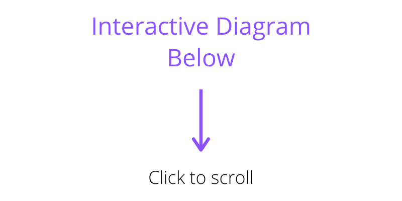
You can check out an interactive demo of the gradient descent algorithm by clicking the image below. Don’t hesitate to play around with it before reading the rest of this article.
In this post, we will go from the fundamentals of optimization, through building an intuition of the math to finally exploring the algorithm and the related consequences. There will be some math, however, it will be limited to the minimum and the key concepts are shown on the figures. However, for a good understanding of the text, I assume you are familiar with derivatives. We will start with the motivation and background for gradient descent.
What is the purpose of gradient descent?
The short answer would be to find a minimum of a function. It is part of the subfield in mathematics called optimisation.
Optimisation is all around us from finding the minimal amount of aluminium needed to make a can or finding the best model which classifies cats and dogs.
The basic approach is to find the minimum directly through functional analysis.
The figure below shows a graphical summary of how we can achieve this.
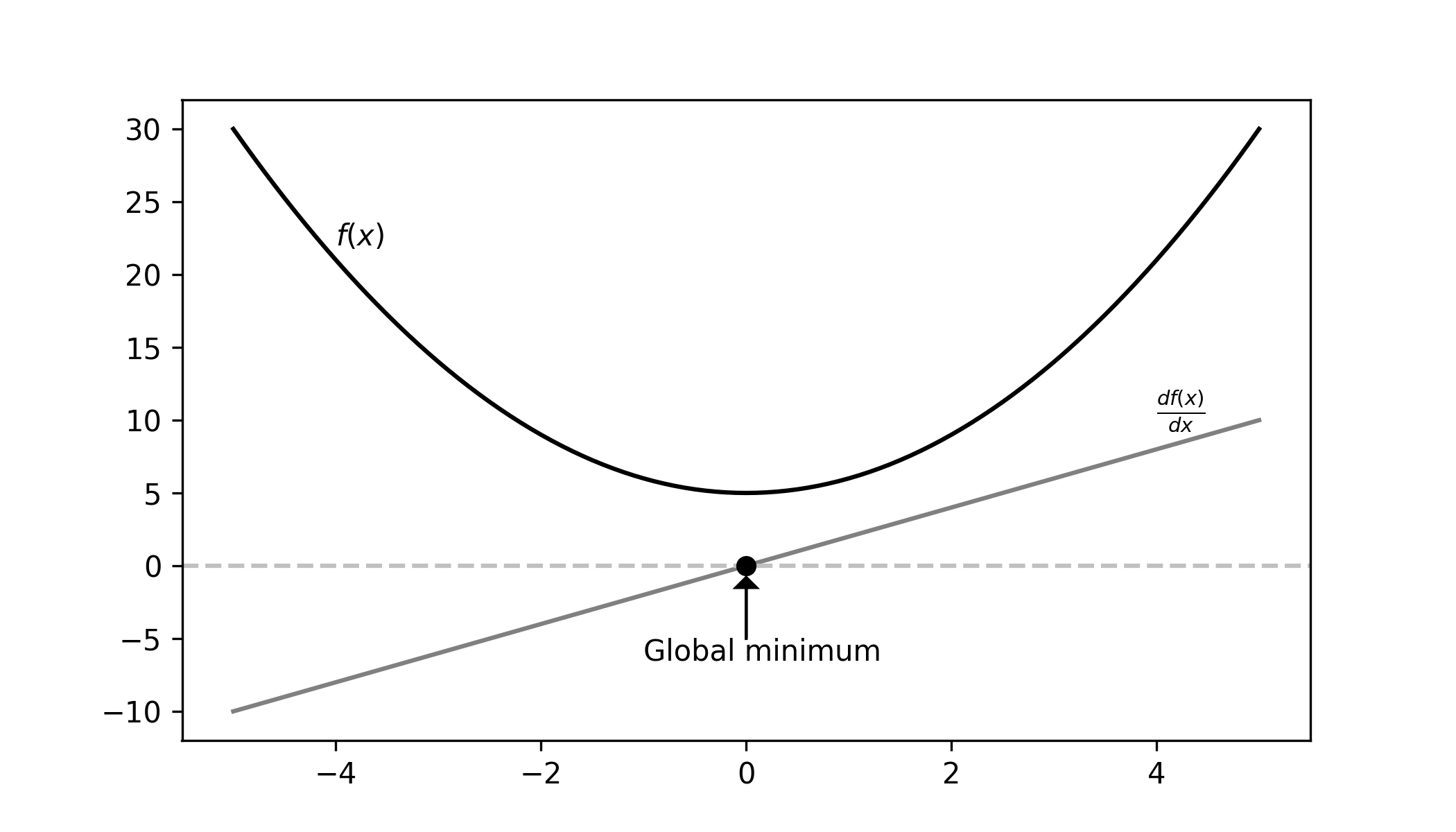
Analytical Minimum
Let’s look at the math step by step. We have a function $f(x)$ (the black line) for which we want to find the minimum. Then we need to do the following steps:
- calculate the derivative $\frac{d f(x)}{dx}$ (the gray line)
- solve $\frac{d f(x)}{dx} = 0$ for $x$ (the black dot)
- check if $x_{min}$ is a minimum (e.g. visually).
Quadratic Example: We will take $f(x) = x^2$. It’s derivative is $2x$. We find the minimal $x$ by finding where $2x$ is equal to $0$. We can immediately see that $x_{min} = 0$ is a solution.
Problems with the analytical solution
Imagine now that the function you want to optimise is $\sin(x)$. The derivative is $\cos(x)$, which is periodic, resulting in infinitely many points where the derivative is $0$. Not mentioning that you have both minimums and maximums! Analytically you can give an expression, which will give you all the minimums:
\begin{align} x_{min} = \begin{cases} 2 \pi n - \frac{\pi}{2}\newline 2 \pi n + \frac{3\pi}{2} \end{cases} \end{align}
However, in Machine Learning we need one particular minimum not all of them. To do this you could limit the function’s domain to e.g. $0 < x < 2\pi$. In this range, you get only $1$ minimum. Unfortunately, this approach has two major problems.
Firstly, we chose a particular domain and we could do so as we know the characteristics of the function. Sadly this is rarely the case and it is unlikely that we would know which domain to choose.
Secondly, we want the lowest possible minimum (ideally the global minimum). In the case of the sine function each minimum has the same value, so it doesn’t really matter. Again this is rarely true in machine learning. More often then not you won’t know where to find the global minimum.
Gradient Descent
A gradient is loosely speaking the same as a derivative. However, there is one conceptual difference. A gradient is considered a vector, not a function. This means that a gradient has a direction. So a gradient at $x$ equal to $-1$ is directed to the left, while the gradient equal to $1$ to the right. You can find a visual representation of the gradient for the quadratic example in the figure below.
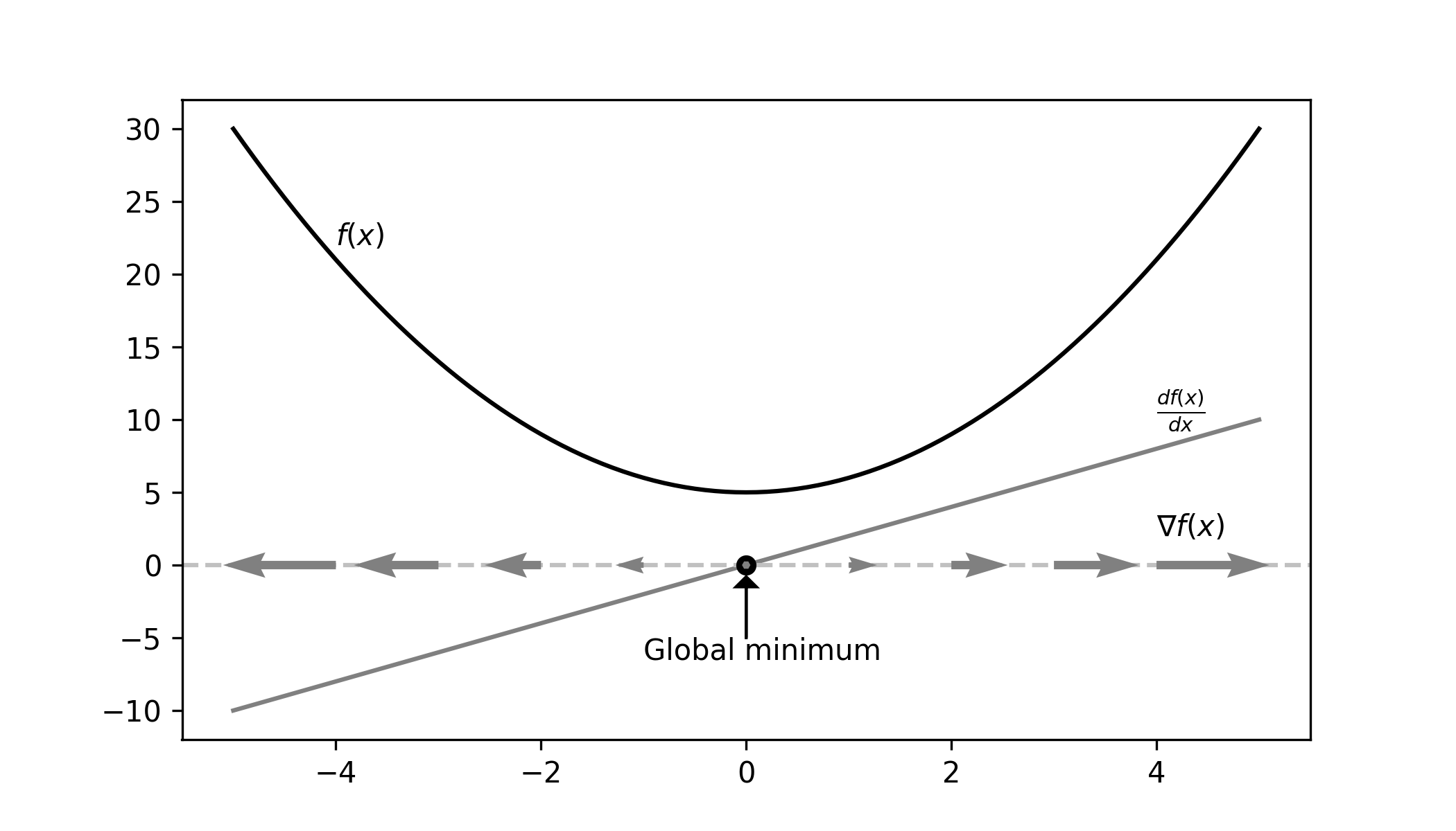
What you might notice is that the gradient is directed away from the minimum. So if we would follow it’s directions we would end up further away from the minimum than when we began.
Imagine you are on a mountain. You see a signpost with a direction for Mount Maximus. However, instead of going to the peak of the mountain, you want to go to the Valley of Minimum. What should you do? Go in the opposite direction! This is where the descent part comes into play.
Gradient Descent
If you go in the opposite direction to the gradient you will reach a minimum.
A Velocity Analogy
In physics, you define movement by at least three parameters. The current position $x$, the velocity $\nabla x$ and the initial position $x_0$. When you want to simulate movement you need to select some time constant $\tau$. It essentially tells us how much time will pass between updates. For example, if $\tau = 1\ s$ then the simulation would tell us would the route would look like if we travelled at the current velocity for $1\ s$. In short, it controls the length of each step. This is essentially simulating a differential equation using the euler approximation method.
Now we can define the position at time $t + 1$ given the position and velocity at time $t$.
\begin{equation} x_{t+1} = x_t + \tau \nabla x_t \end{equation}
You can observe that when simulating movement the body essentially follows the velocity gradient $\nabla x_t$. So we can use the same approach to run gradient descent if we use $-\nabla f(x)$ as the velocity. You need to add the minus to move in the opposite direction to the gradient. This means that we can see gradient descent as movement against the gradient.
The Gradient Descent Algorithm
Now that we have everything in place we can define the gradient descent algorithm.
\begin{equation}\label{eq:gradient_descent} x_{t+1} = x_t - \eta \nabla f(x_t) \end{equation}
In Machine Learning instead of calling $\eta$ a time constant it is called the learning rate. The expression $\eta \nabla f(x_t)$ is also known as the delta as it is the de facto change in $x$. Precisely the gradient descent algorithm can be given as follows:
- Select an initial position $x_0$ and learning rate $\eta$
- Update the position $x$ according to equation \ref{eq:gradient_descent}
- Repeat step 2. until convergence (e.g. until $\nabla f(x_t)$ becomes very small).
Interactive Demo
You can try out the algorithm in the demo below. By now you should know what the first two parameters are responsible for. We will go into detail with the remaining two in the following sections. Try to build an intuition as to what are the consequences of different settings. What happens if the learning rate is too high or too low? Can you converge from every initial position? Can you see some problems with the algorithm?
function:
Local Minimum
One of the biggest problems is the gradient descent doesn’t guarantee that it will converge to a global minimum. So we can only be sure that we converge to some minimum, which likely will be a local minimum. You can visualise this if you look at the local function in the simulation. Also, the figure below shows you an example of a local and global minimum.
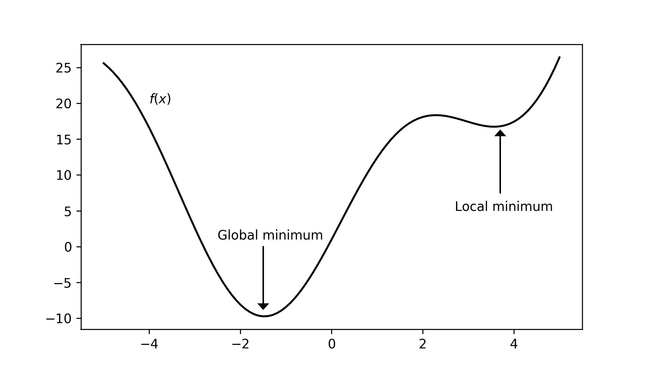
This is a common problem in machine learning, where your algorithm might have converged, but it is not found the best possible solution. So let’s look at different methods to find a better minimum.
Random Initialization
One option is to simply run gradient descent multiple times with different initial positions and select the solution which ends up in the lowest point. This will be quicker than randomly sampling every point individually to brute force the minimum, as many points converge to the same positions. You can see this in the demo by sliding the $x_0$ slider. However, this also will not guarantee the global minimum, but we should end up with a better minimum.
Learning Rate Decay
This method suggests to keep taking smaller steps. It is meant to prevent oscillations, which can result in skipping the minimum. In addition with ever-smaller steps, we have a chance of squeezing into a narrower minimum, which normally would be jumped over. See the notch function in the demo. Another idea is that we can start with a larger learning rate skipping through potentially most of the local minimums and then continue with a more steady rate. To incorporate decay we add an extra step in our algorithm.
\begin{equation} \eta_{t+1} = \eta_t \cdot \eta_{decay} \end{equation}
At every iteration, we multiply the learning rate by a $\eta_{decay}$ parameter. This method doesn’t guarantee a global minimum, but it can help reach a better local minimum.
Momentum
Imagine you roll a ball down a hill. It doesn’t stop immediately as it reaches the bottom, but rather it keeps rolling back and forth. If there is a small indent on the way (a local minimum) it will roll right through. This is due to momentum and the idea is to apply the same process to gradient descent.
First we will need to store the “velocity” $\nabla f(x_{t-1})$ at the previous step. Now in the next step, we need to also tackle a fraction of the velocity we previously had. You can choose the size of this fraction, which we will call $\beta$. With this in mind we can modify equation \ref{eq:gradient_descent} to be:
\begin{align} x_{t+1} &= x_t\newline &+ \beta \nabla f(x_{t-1})\newline &- \eta \nabla f(x_t) \end{align}
Now, this allows us to “jump” out of some local minimums. Unfortunately, we again will not get a guarantee of reaching the global minimum.
Can we ever be sure that we will reach the global minimum?
In the case of gradient descent, it is possible. However, it depends on the function you are optimizing. If it is a convex function (like $x^2$) than you could be sure, but if the functions become more complicated then it depends. A big part of machine learning is to find algorithms and functions, which can guarantee a global minimum. However, although gradient descent doesn’t always guarantee a global minimum it does give us a minimum. This is better than nothing! In fact finding a good (but not necessarily the best) minimum is usually sufficient making gradient descent one of the most widely used algorithm in machine learning.
Relationship to Machine Learning
I have repeatedly mentioned that gradient descent is used in machine learning. The question is why? Why do we need optimisation in machine learning? In machine learning, we build models, which are able to predict data. We then define functions called loss functions which measure how bad is this prediction. You want the model which is the least bad, meaning you want to find parameters which minimize the loss function. To do this you may use gradient descent.
Conclusion
Hopefully, after reading this you have a better understanding of gradient descent. The key point that you should take away from this post is that:
Gradient descent is a numerical method of finding the minimum of a function.
The next step from here would be to look at loss functions and then tackle linear regression. There are also other flavours of gradient descent like Stochastic Gradient Descent or Batch Gradient Descent. Make sure to check those out as well!
If you found this article helpful, share it with others so that they can also have a chance to find this post. Also, make sure to sign up for the newsletter to be the first to hear about the new articles. If you have any questions make sure to leave a comment or contact me directly.
Want more resources on this topic?
Citation
Cite as:
Pierzchlewicz, Paweł A. (Sep 2020). What is gradient descent?. Perceptron.blog. https://perceptron.blog/gradient-descent/.
Or
@article{pierzchlewicz2020gradientdescent,
  title   = "What is gradient descent?",
  author  = "Pierzchlewicz, Paweł A.",
  journal = "Perceptron.blog",
  year    = "2020",
  month   = "Sep",
  url     = "https://perceptron.blog/gradient-descent/"
}