
Hodgkin-Huxley Model
Quantifying the activity of a neuron

Interactive Demo
The left plot shows the input current and the right one shows the membrane voltage. Upon increasing the input current you can observe that the membrane potential begins to exhibit spiking behaviour.
Read More
Back in 1952 Hodgkin and Huxley found that there are three main types of currents describing the dynamics of a neuron: Sodium (N), Potassium (K), and a leak current, which mostly consists of Calcium (Cl). The flow of these ions is controlled by voltage-gated ion channels. They are biological constructs in the membrane of a neuron that gate the flow of specific ions depending on the membrane potential. When the neuron’s membrane reaches a certain voltage they open up allowing these ions to move in and out of the neuron.
| link | description |
|---|---|
| Numpy implementation of the Hodgkin-Huxley model. | |
| Numpy implementation of the |
The code for this project is available on Github .
Basics of ion flows
The cell membrane is impermeable to ions.
The fundamental element that we first need to understand is the cell membrane. It is a barrier discriminating between the inside and outside of a cell. Its feature that will interest us most is that it is mostly impermeable to ions. As a result, it acts as a capacitor.
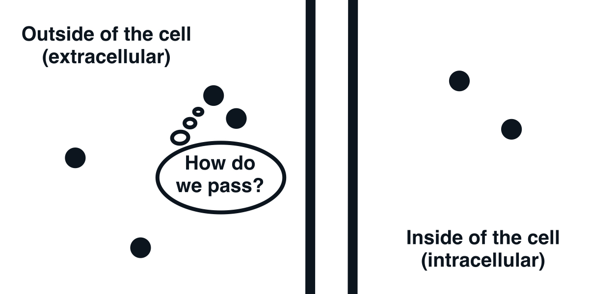
The cell membrane is impermeable to ions.
Ion Channels allow ions to pass the cell membrane.
Since the membrane is mostly impermeable to ions, there has to be a mechanism that lets them in and out. This is the prime role of ion channels. You can think of them as small holes in the membrane, which sometimes open up allowing the flow of ions. First, let’s just consider they are always open and discuss the flow then.
Two forces are acting on the ions: electrical and chemical. The intracellular concentration of ions is significantly different from the extracellular. Ions want to negate this difference, so the ions from the higher concentration compartment flow to the lower concentration compartment. This movement of ions is credited to the chemical force arising from the chemical gradient. Since there are different concentrations of ions, which are associated with different charges, you can also observe a difference in electrical potentials between the intracellular area and extracellular. Due to Coulomb’s law, this results in an electrical force. These forces act in opposite directions counteracting each other.
An interesting property of single ion systems is the Nernst potential. Take a hypothetical two-compartment system where there is only one ion type. Can we apply another force that will stop the flow of ions between the compartments? It turns out that by applying a potential difference of the appropriate strength between the two compartments then the flow is at equilibrium. At this point the electrical and chemical forces are equal and this potential is called the Nernst potential or reversal potential.
However, ion channels are not always open. They are mostly closed and open only in very specific conditions. Here we will only look at the voltage-gated ion channels, which only open up when the membrane potential is high enough. The precise timing of when each ion channel opens is important to generate spikes and we will discuss this in more detail a bit later.
A circuit representation of a neuron
Given the knowledge of the neurophysiology of a neuron, we can build a circuit model of a neuron. This will require adding a capacitor, an input current, and each ion channel as a serially connected resistor (gating) and battery (driving force). The diagram of the neuron can be found below.
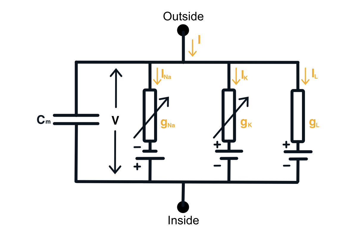
Hodgkin-Huxley circuit model of a neuron.
Now we would want to find out how to compute the membrane voltage. We can do this using the 1st Kirchhoff’s Law we can write down the equation for the currents in this circuit. You can notice that the input current splits into the current through the capacitor and the current through all the ion channels. \begin{equation} I(t) = I_C(t) + \sum_k I_k(t) \end{equation} Then using the definition of the current across the capacitor, we can get the differential equation for the membrane voltage. \begin{equation} C \frac{du}{dt} = - \sum_k I_k(t) + I(t) \end{equation}
Channels are gated by voltage
Each of the ion currents describes the flow of the ion type through its corresponding channel. Assuming the channel is completely open the current is described by Ohm’s law. The potential is the membrane potential decreased by the ion’s reversal potential and the conductance arises from the limited carrying capacity of the channel.
However, we also have a parameter that we will call the probability that the channel is open, which is a function of voltage and it determines the dynamics of the channel. \begin{equation} I_k = P(u) g_k (u - E_k) \end{equation} These probabilities are described by a set of parameters $p$ (activation parameters $n$, $m$, and an inactivation parameter $h$). These parameters are each described by a differential equation. For the activation parameters, it is \begin{equation} \frac{dp}{dt} = \alpha_p(u) (1-p) - \beta_p(u) p \end{equation} and for inactivation, it is given as \begin{equation} \frac{dp}{dt} = \beta_p(u) (1-p) - \alpha_p(u) p \end{equation} Here $\alpha$ and $\beta$ are Boltzmann equations describing the stochastic behavior of the channels and have the general form \begin{align} \alpha_p(u) &= \frac{\theta_{p, 1} (u - \theta_{p, 2})}{\theta_{p, 4} - \exp\left(\frac{\theta_{p, 2} - u}{\theta_{p, 3}}\right)} \newline \beta_p(u) &= \theta_{p, 5} \exp\left(-\frac{u}{\theta_{p, 6}}\right) \end{align} The $\theta_p$ values were found experimentally to best exhibit the behavior of a neuron. Finally, the parameters $h$, $m$, and $n$ construct the probability of the channel being open in the following way \begin{align} P_K &= n^4 \newline P_{Na} &= m^3 h \end{align} and the leak channel is always open.
Simulating the neuron
Having defined the channel dynamics we can finally determine the algorithm for simulating a neuron by approximating the differential equations using the forward Euler approximation.
1
2
3
4
5
6
7
8
9
10
11
12
13
14
15
16
17
18
19
20
21
22
23
24
25
26
27
28
29
30
31
32
33
34
35
36
37
38
39
40
41
42
43
44
45
46
47
48
49
50
51
52
53
54
55
56
57
58
59
60
61
62
63
64
65
import numpy as np

class SingleCompartmentModel(object):
    def __init__(
            self,
            C_m=1,
            E_Na=115,
            E_K=-12,
            E_L=10.6,
            E_m=0,
            g_Na=120,
            g_K=36,
            g_L=0.3
    ):
        self.C_m = C_m
        self.E_Na = E_Na
        self.E_K = E_K
        self.E_L = E_L
        self.E_m = E_m
        self.g_Na = g_Na
        self.g_K = g_K
        self.g_L = g_L

        self.m_params = [1, 0.1, 25, 10, 1, 4, 18]
        self.n_params = [0.1, 0.01, 10, 10, 1, 0.125, 80]
        self.h_params = lambda u: [.5, 1/(30 - u), 30, 10, -1, 0.07, 20]

        self.m_0 = 0.0529
        self.h_0 = 0.5646
        self.n_0 = 0.3145

    @staticmethod
    def alpha(V, params):
      return params[1] * (V - params[2]) / (params[4] - np.exp(-(V - params[2]) / params[3]))

    @staticmethod
    def beta(V, params):
      return params[5] * np.exp(- V / params[6])

    def response(self, I_e, start=-200, end=600, dt=0.025):
        ts = np.arange(start, end, dt)

        I = np.zeros(len(ts))
        V = np.zeros(len(ts))

        m = np.ones(len(ts)) * self.m_0
        h = np.ones(len(ts)) * self.h_0
        n = np.ones(len(ts)) * self.n_0

        for step, t in enumerate(ts[:-1]):
            I[step] = I_e(t)

            I_L = self.g_L * (V[step] - self.E_L)
            I_Na = self.g_Na * m[step] ** 3 * h[step] * (V[step] - self.E_Na)
            I_K = self.g_K * n[step] ** 4 * (V[step] - self.E_K)

            V[step + 1] = dt / self.C_m * (I[step] - I_L - I_Na - I_K) + V[step]

            h_params = self.h_params(V[step])
            h[step + 1] = dt * (self.beta(V[step], h_params) * (1 - h[step]) - self.alpha(V[step], h_params) * h[step]) + h[step]

            m[step + 1] = dt * (self.alpha(V[step], self.m_params) * (1 - m[step]) - self.beta(V[step], self.m_params) * m[step]) + m[step]
            n[step + 1] = dt * (self.alpha(V[step], self.n_params) * (1 - n[step]) - self.beta(V[step], self.n_params) * n[step]) + n[step]

        return ts, V, I, m, h, n
Model Parameters
| Parameter | $\theta_1$ | $\theta_2$ | $\theta_3$ | $\theta_4$ | $\theta_5$ | $\theta_6$ |
|---|---|---|---|---|---|---|
| $h$ | $\frac{1}{30 - u}$ | 30 | 10 | -1 | 0.07 | 20 |
| $m$ | 0.1 | 25 | 10 | 1 | 4 | 18 |
| $n$ | 0.01 | 10 | 10 | 1 | 0.125 | 80 |
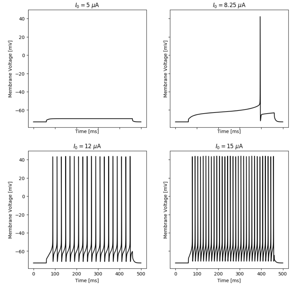
By simulating the neuron we can observe that the membrane potential begins to generate action potentials (spikes) once the input current increases above a certain threshold. We can visualize the membrane potential at different input currents as shown below. Additionally, we can look at the steady-state spiking rate of the neuron.
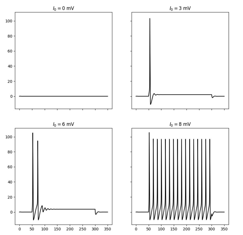
Responses of the simulated neuron at different input currents.
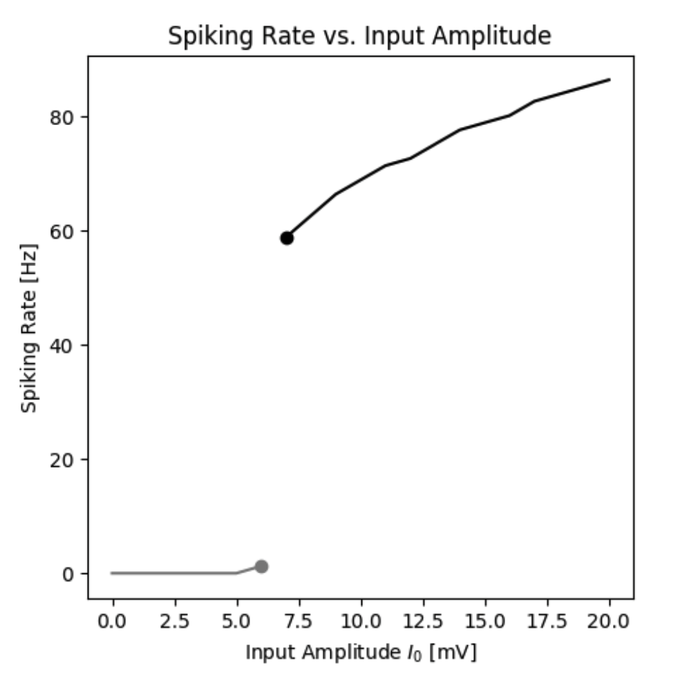
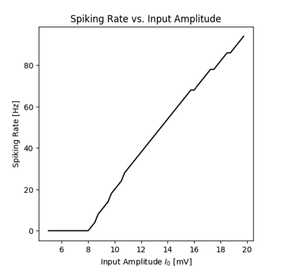
Spiking rate of a neuron as a function of the input current.
Firing rate as a function of input current
By simulating the neuron we can observe that the firing rate of the neuron is a function of the input current. In this standard model the firing rate $r(I)$ could be approximated by a Heaviside function. However, different types of functions can be obtained by different neuron types.
ReLU-type behavior with an A-type Potassium current
A different type of response pattern can be obtained by adding an A-type current to the neuron. The A-type current is an additional potassium current that is not present in the original model. Its open state is defined by the channel opening probability $P_A = a^3b$ and the channel conductance $g_A$.
Adding this extra potassium current changes the relationship between the firing rate and input current. With this current, it is no longer a Heaviside, but instead, it becomes a linear threshold function also known as the rectified linear function (ReLu).
Responses of the simulated neuron with an A-Type current at different input currents.
Spiking rate of a neuron with an A-Type current as a function of the input current.
The inspiration for artificial neural networks
Based on the activation of the neuron you can observe that there are two states: firing and not firing. The firing state can be defined by the activation function $f(I)$. In the case of the standard model, the activation function is a Heaviside function, while the model with the A-Type current has a ReLU function. The idea is that the inputs $I_i$ are summed by the neuron and the final firing rate is the result of passing the sum through an activation function $f$. \begin{equation} r(\mathbf{I}) = f\left(\sum_i^N I_i \right) \end{equation} This abstraction was used to move from the complex and computationally expensive model to a simpler and cheaper rate-based model. As a result, making it easier to model networks of neurons. This transition has formed the basis for the now very popular artificial neural networks.
Want more resources on this topic?
Citation
Cite as:
Pierzchlewicz, Paweł A. (Nov 2022). Hodgkin-Huxley Model. Perceptron.blog. https://perceptron.blog/hodgkin-huxley/.
Or
@article{pierzchlewicz2022hodgkinhuxley,
  title   = "Hodgkin-Huxley Model",
  author  = "Pierzchlewicz, Paweł A.",
  journal = "Perceptron.blog",
  year    = "2022",
  month   = "Nov",
  url     = "https://perceptron.blog/hodgkin-huxley/"
}