
Langevin Monte Carlo: Sampling using Langevin Dynamics
How to sample from a distribution using Langevin Dynamics and why it works.

Generative models rely on the ability to sample from a distribution. When the distribution is known the task of sampling from it is straightforward, for example, sampling from a normal distribution. However, in many applications (e.g. generating images of human faces) the distribution can be difficult to express explicitly, and computing the exact distribution is intractable. Therefore, methods like Markov Chain Monte Carlo (MCMC) are used, which allow sampling from a distribution without the need to explicitly compute it. Langevin Monte Carlo is an MCMC method that uses Langevin Dynamics to sample from a distribution.
Here this blog post will explain the basics of Langevin Monte Carlo exploring how and why it works. We will first delve into the theory of Langevin Dynamics and how it relates to Markov Chain Monte Carlo. Next, we will show that using Langevin Dynamics we can generate samples from the distribution that we are interested in. Finally, we will show how to use Langevin Dynamics to sample from a distribution.
What are Langevin Dynamics?
Langevin Monte Carlo relies on Langevin Dynamics to sample from a distribution. Langevin Dynamics describes the evolution of a system that is subject to random forces. Originally, Langevin Dynamics were used to describe Brownian motion. The Langevin Equation for Brownian motion is: \begin{equation} m \ddot{x} = -\lambda \dot{x} + \eta \end{equation} where $m$ is the mass of the particle, $\lambda$ is the damping coefficient, $\eta \sim \mathcal{N}(0, 2\sigma^2)$ is a Gaussian noise with zero mean and variance $2\sigma^2$, and $t$ is the time.

On a particle of mass $m$ acts a random force $\vec{F}$
We can transform this in terms of potential energy $V(x)$ and define it as the velocity of the particle. First we note that the LHS is the definition of the force $F$ acting on the particle, which is equal to the change in the potential energy of the system. \begin{equation} m \ddot{x} = F = \frac{\partial V(x)}{\partial x} = \nabla V(x) \end{equation} By substituting the change in potential energy $V(x)$ we notice that the equation describes the evolution of the force $F$ acting on the particle. \begin{equation} \nabla V(x) = -\lambda \dot{x} + \eta \end{equation} We can rearange the equation to get the equation to obtain a differential equation describing the evolution of the position $x$ of the particle. \begin{equation} \lambda \dot{x} = -\nabla V(x) + \eta \end{equation} which now we can rewrite as a Stochastic Differential Equation (SDE): \begin{equation} dx = -\nabla V(x) dt + \sqrt{2}\sigma dW \end{equation} where $-\nabla V(x)$ is the drift term, $\sigma$ is the volatility, and $dW$ is a time-derivative of a standard Weiner process.
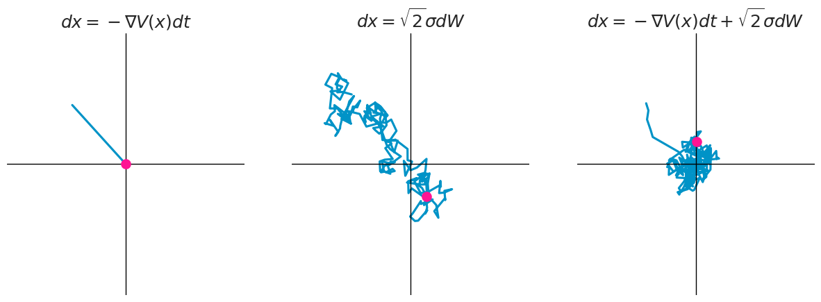
Decomposition of Langevin dynamics. From the left: only potential energy, only random force, both combined.
Deriving the Steady State of Langevin Dynamics
To show how to use the Langevin Equation to sample from a distribution we need to identify the distribution $q(x, t)$ that the Langevin Equation generates. In particular we are interested in a steady state distribution $q_\infty(x)$. For this, we shall turn to the Fokker-Planck equation, which is a partial differential equation that describes the time evolution of a probability density function. The Fokker-Planck equation is defined for a typical SDE in the form: \begin{equation} dx = \mu(x,t) dt + \sigma(x, t) dW \end{equation} where $\mu(x,t)$ is the drift term, $\sigma(x, t)$ is the volatility. We define the diffusion coefficient as: $D(x, t) = \sigma(x, t)^2 / 2$. For such SDE the Fokker-Planck equation is: \begin{equation} {\frac {\partial }{\partial t}}p(x, t)=-{\frac {\partial }{\partial x}\left[\mu (x,t)p(x,t)\right]+{\frac {\partial ^{2}}{\partial x^{2}}}\left[D(x,t)p(x,t)\right].} \end{equation} Thus for our SDE we have: \begin{equation} {\frac {\partial }{\partial t}}q(x, t)={\frac {\partial }{\partial x}\left[\nabla V(x) q(x,t)\right]+{\frac {\partial ^{2}}{\partial x^{2}}}\left[\sigma^2 q(x,t)\right].} \end{equation}

Simulation of the Fokker-Planck equation. Shows the evolution of the distribution $q(x, t)$ over time. Here the initial distribution is a mixture of two Gaussian distributions, and the drift is selected such that a Gaussian distribution is generated. As you can see the distribution after some time becomes constant (~250 steps).
Now to obtain the steady state distribution we have to solve for ${\frac {\partial }{\partial t}}q(x, t) = 0$. Thus for the steady-state distribution we define: \begin{equation} {\frac {\partial }{\partial t}}q_\infty(x)=\frac{\partial}{\partial x}\left[\nabla V(x) q_\infty(x) + \frac {\partial}{\partial x}\left[\sigma^2 q_\infty(x)\right]\right] = \frac{\partial}{\partial x} J = 0 \end{equation} Where $J$ is the probability current. The probability current describes the flow of a probability given the space $x$. We impose a condition on the distribution, such that the probability current is zero at infinity. Since the derivative of the flux is zero this means that it is constant and thus $J(x) = 0$ for all $x$. As a result, we obtain the following differential equation: \begin{equation} \frac{\partial}{\partial x} q_\infty(x) = -\frac{\nabla V(x)}{\sigma^2} q_\infty(x) \end{equation} which we can solve obtaining: \begin{equation} q_\infty(x) \propto \exp\left(-\frac{V(x)}{\sigma^2}\right) \end{equation} Thus in the special case when $\sigma = 1$ we obtain the following distribution: \begin{equation} q_\infty(x) \propto \exp\left(-V(x)\right) \end{equation} which means that if we want to sample from the distribution $p(x)$ we need to set the potential energy to be \begin{equation} V(x) = -\log(p(x)) \end{equation} Note that in the case that the $\sigma \ne 1$, by setting the potential energy as defined above we would obtain a distribution with altered variance. For example, consider that $p(x)$ is a Gaussian distribution with zero mean and variance $\sigma_n^2$. Then for $\sigma = 1$ we obtain $q_\infty(x) = \frac{1}{Z} \exp\left(-\frac{x^2}{\sigma_n^2}\right)$. Which is the same as the Gaussian distribution with zero mean and variance $\sigma_n^2$. However, for $\sigma \neq 1$ we obtain \begin{equation} q_\infty(x) = \frac{1}{Z} \exp\left(-\frac{x^2}{\sigma^2\sigma_n^2}\right), \end{equation} which would be a gaussian with the variance modified by $\sigma^2$.
Sampling Using Langevin Dynamics
Having shown that Langevin Dynamics converge to the desired distribution in the steady state we are now positioned to ask how to sample from the distribution. Let’s rewrite the Stochastic Differential Equation in terms of the target distribution $p(x)$. \begin{equation} dx = \nabla \log p(x) dt + \sqrt{2}\sigma dW \end{equation} We can use the Euler-Maruyama method to numerically approximate the solution to this equation. According to the Euler-Maruyama method we recursively compute:
\begin{equation} x_{n+1} = x_n +\nabla \log p(x_n) \epsilon + \sqrt{2}\sigma \Delta W \end{equation}
where $\epsilon$ is the time step and $\Delta W \sim \mathcal{N}(0, \epsilon)$ is a normal random variable with zero mean and $\epsilon$ variance. We can thus rewrite in terms of $z \sim \mathcal{N}(0, 1)$ obtaining: \begin{equation} x_{n+1} = x_n + \nabla \log p(x_n) \epsilon + \sigma \sqrt{2 \epsilon}\ z \end{equation}
Below is an example of the time evolution of the distribution $q(x, t)$ for a Gaussian distribution with zero mean and unit variance approximated using the Euler-Maruyama method.
Implementation for the above simulation excluding the plotting code.
1
2
3
4
5
6
7
8
9
10
11
12
13
14
15
16
17
18
19
20
import torch
import torch.distributions as D

eps = 0.01
steps = 500
n_samples = 10000

# d/dx -log p(x) for N(0, 1)
force = lambda x: -x

# Prior distribution from which the initial positions are sampled
prior = D.Uniform(torch.Tensor([-10, -10]), torch.Tensor([10, 10]))

# Run Langevin Dynamics
x = prior.sample((n_samples, ))
for i in range(steps):
    x = x + eps * force(x) + torch.sqrt(2 * eps) * torch.randn(size=x.shape)

x.mean().item(), x.std().item()
# >>> something close to (0.0, 1.0)
Want more resources on this topic?
Citation
Cite as:
Pierzchlewicz, Paweł A. (Jul 2022). Langevin Monte Carlo: Sampling using Langevin Dynamics. Perceptron.blog. https://perceptron.blog/langevin-dynamics/.
Or
@article{pierzchlewicz2022langevindynamics,
  title   = "Langevin Monte Carlo: Sampling using Langevin Dynamics",
  author  = "Pierzchlewicz, Paweł A.",
  journal = "Perceptron.blog",
  year    = "2022",
  month   = "Jul",
  url     = "https://perceptron.blog/langevin-dynamics/"
}