
What is linear regression?
On fitting a line to your data

Linear Regression (LR) is one of the most fundamental algorithms in machine learning. It is the simplest regression model out there it is very often a fitting solution for a lot of problems. On top of that, LR is a great introductory model for explaining a lot of machine learning concepts. However, most definitions out there aren’t always very intuitive for newcomers into the field.
Linear regression is simply finding the best line which fits the data.
With this post, I want to provide an intuitive yet complete explanation of LR. This post turned out to be a bit more on the mathy side of things; however, it was necessary to show all the exciting features of LR.
Below you can find a demo of linear regression. Click the button to run the simulation and to reset the parameters.
The linear model has to fit to the data. You can see that it aligns with the slope of the data. At the same time the orange error begins decreases. On the right you can see the evolution plots for the weight parameter and the variance. The dashed line indicates the true values.
Read More
What I expect you to know
Since this is a bit more mathy I suggest you should know the following concepts. However, do not worry if you are not super confident with them. We will go through everything step by step avoiding magic jumps!
- Basic linear algebra, vectors and matrices.
- Basic calculus, derivatives should not be something terrifying.
- Probability theory, you should know the Gaussian/Normal distributions and the product rule.
If you want to get better with math necessary for machine learning, make sure to look at this great book on just that Mathematics for ML. I also have some previous posts that I refer to in this post, that you might want to read first.
Linear? Regression!?
Before we jump into some examples and some math lets decompose the algorithm’s name to understand what it means. It has two components linear and regression.
Linear as in like a line
Linear in Linear regression refers to the type of model/function that we want to fit. In this case, it is a linear function, which takes the form of: \begin{equation} \color{purple}{f}(\color{orange}{x}) = a\color{orange}{x} + b \end{equation} If you plotted this function you would get a line, where the slope and the intersection with the y-axis is controlled by $a$ and $b$. In linear regression, we would call $a$ and $b$ the parameters of the model, as we would be adjusting them such that they best represent the data.
Regression as in predicting the value
In machine learning, we have different types of tasks. The simplest to explain is the classification task. Say you are looking at a bunch of houses that you want to buy. You show a classification model a house with a size of $500 m^2$, and it will tell you that it is a mansion. Then you show it an apartment that is $20 m^2$, and it will tell you that it is a studio.
Regression is another example of a machine learning task. However, instead of predicting the classes, it gives direct values. Let’s consider the two houses again. Now instead of giving you a class, it will return a predicted price. For example, the $500 m^2$ it might return 5 mln USD and for the $20 m^2$ 200k USD.
Use-case: Predicting House Prices
Following the example of searching for houses, we can look at how we can apply linear regression to predict house prices. Say you want to sell your house, but you don’t know what price you should demand. To get an estimate, you go to your favourite real estate website (obviously everyone has one, right?) and download all of the sales offers from your area. Your first idea is that the size of the house has to determine the price and you get something like the plot below.
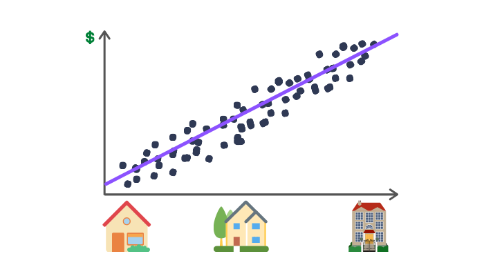
You notice that the larger the house the higher the price and that it (conveniently) looks roughly like a line. Now you want to know how much you can get for your house, which is $121.2 m^2$. You could average out all the offers with the same area but say none is exactly $121.2 m^2$. Should you average the prices of offers between $121 m^2$ and $122 m^2$? Or maybe $100 m^2$ and $200 m^2$? Selecting this range would be a pain, and instead, we can use the fact that the data lies nicely on a line and just fit a linear function! You notice that a line with a slope of 10k USD best fits the data. With that, you can compute that you should demand 1.212mln USD for your house. Now we managed to guess this, but it would be nice to do this automatically.
The math of linear regression
We will now dive into the math, feel free to skip this part directly to the implementation.
One can assume that the data follow some linear function with some noise overlayed on top. Since we don’t know much about the noise, we can assume it is normally distributed or in other words that it is white noise. By definition, white noise doesn’t introduce bias (the mean of the noise is $0$). Thus we can write down the function that we think models how the data is generated. \begin{equation} \color{purple}{y}(\color{orange}{x}) = w\color{orange}{x} + \color{purple}{\mathcal{N}}(0, \sigma^2) \end{equation} Here we will assume that there is no bias component for simplicity, but later I will show you how simple it is to add this component. Adding a deterministic (not random) variable to a normal distribution shifts the mean. As a result we assume that the data is sampled from the following distribution: \begin{equation} Y \sim \color{purple}{\mathcal{N}}(wx, \sigma^2) \end{equation}
Likelihood
For this distribution we can define the likelihood of the random variable $y$ for a given $x$. \begin{equation} \color{purple}{p}(\color{orange}{y_i} \mid \color{orange}{x_i}) = \frac{1}{Z \sigma} \color{purple}{\exp}\left(-\frac{1}{2} \frac{(w\color{orange}{x_i} - \color{orange}{y_i})^2}{\sigma^2}\right) \end{equation} Here $Z$ is a normalisation parameter which ensures that the likelihood sums to $1$. This is the likelihood for each data point. The product rule allows us to get the general likelihood for the entire dataset. \begin{equation} \color{purple}{p}(\color{orange}{\mathbf{y}} \mid \color{orange}{\mathbf{x}}) = \prod^N_{i=0} \frac{1}{Z\sigma} \color{purple}{\exp}\left(-\frac{1}{2} \frac{(w\color{orange}{x_i} - \color{orange}{y_i})^2}{\sigma^2}\right) \end{equation} With this likelihood defined we can define an optimisation problem as finding such parameters $w$, which maximise the likelihood. \begin{equation} \arg\max_w \color{purple}{p}(\mathbf{y} \mid \mathbf{x}) \end{equation} However, optimising likelihood is not the most forgiving since the derivative of products is difficult to compute. Instead we can compute the log-likelihood exploiting the product to sum property of logarithms \begin{equation} \color{purple}{\ln}\left(\prod_{i=0}^N a_i\right) = \sum_{i=0}^N \color{purple}{\ln}(a_i) \end{equation} and that \begin{equation} \arg\max_w \color{purple}{p}(\mathbf{y} \mid \mathbf{x}) = \arg\max_w \color{purple}{\ln} \color{purple}{p}(\mathbf{y} \mid \mathbf{x}) \end{equation} As a result the following log-likelihood is obtained. Note that we dropped the optimisation parameter $Z$ as it is does not influence the outcome of the algorithm. \begin{equation} \color{purple}{\ln p}(\color{orange}{\mathbf{y}} \mid \color{orange}{\mathbf{x}}) = -\left(N\color{purple}{\ln}{\sigma} + \sigma^{-2} \underbrace{\frac{1}{2} \sum^N_{i=0} (w\color{orange}{x_i} - \color{orange}{y_i})^2}_{\text{MSE}}\right) \end{equation} You might notice that the part inside the bracket is just the mean squared error (MSE) loss! This may become more apparent when we note that usually for linear regression, we assume variance of the system $\sigma^2 = 1$. At this point it should be clear that the log-likelihood is just the negative of MSE. \begin{equation} \color{purple}{\ln p}(\color{orange}{\mathbf{y}} \mid \color{orange}{\mathbf{x}}) = -\left(\underbrace{\frac{1}{2} \sum^N_{i=0} (w\color{orange}{x_i} - \color{orange}{y_i})^2}_{\text{MSE}}\right) \end{equation}
Loss function
Thus we can see that using the negative of the log-likelihood as a loss function makes sense. \begin{equation} \color{purple}{L}(\color{orange}{w}, \color{orange}{\sigma}) = - \color{purple}{\ln p}(\mathbf{y} \mid \mathbf{x}) \end{equation} However, for our considerations we will keep $\sigma$ as a parameter so that you can understand why we set it to $1$. All in all, based on the above considerations, the likelihood is maximised when MSE is minimised. Thus we will minimise the following loss function. \begin{equation} \color{purple}{L}(\color{orange}{w}, \color{orange}{\sigma}) = N\color{purple}{\ln}{\color{orange}{\sigma}} + \frac{1}{2\color{orange}{\sigma}^2} \sum^N_{i=0} (\color{orange}{w}x_i - y_i)^2 \end{equation} To make this actually MSE we will divide the loss by $N$. This will ensure that the loss is independent of the number of data points. We can do this because scaling a function by a constant doesn’t change the position of an extremum. \begin{equation} \color{purple}{L}(\color{orange}{w}, \color{orange}{\sigma}) = \color{purple}{\ln}{\color{orange}{\sigma}} + \color{orange}{\sigma}^{-2}\frac{1}{2N} \sum^N_{i=0} (\color{orange}{w}x_i - y_i)^2 \end{equation} Knowing that this model has two parameters $w$ and $\sigma$ we will have to optimise the loss for each of them.
Optimising the weights
We will start with $w$ as it is the parameter that controls the line’s shape that we are fitting. To optimise this we compute the partial derivative of the loss function with respect to $w$. \begin{equation} \frac{\partial \color{purple}{L}(\color{orange}{w}, \color{orange}{\sigma})}{\partial w} = \frac{1}{N\color{orange}{\sigma}^2} \left(\color{orange}{w}\mathbf{x}\mathbf{x}^\top - \mathbf{y}\mathbf{x}^\top\right) \end{equation} Note that the derivative is dependent on both $w$ and $\sigma$, however given that we can factor out $\sigma$ it’s role is purely to scale the gradient. Further, since this is a partial derivative, we assume $\sigma$ to be a constant. Thus following from the definition of the gradient descent algorithm, we can absorb $\sigma$ into the learning rate $\eta_w$. With this in mind we can define the update rule for $w$. \begin{equation} w_{t + 1} \leftarrow w_t - \eta_{w} \left(w\mathbf{x}\mathbf{x}^\top - \mathbf{y}\mathbf{x}^\top\right) \end{equation} You can notice that as a result this update rule is independent of $\sigma$. This means that regardless of the value that $\sigma$ takes the weight $w$ will converge to the same solution. For linear regression, you can provide an explicit solution by setting the derivative to $0$. As a result we get: \begin{equation} w^* = (\mathbf{x}\mathbf{x}^\top)^{-1}\mathbf{y}\mathbf{x}^\top \end{equation} Notice that the explicit solution will not depend on $\sigma$, so this further justifies setting $\sigma = 1$. Here most linear regression derivations end, with the update rule and explicit solution. However, we have considered $\sigma$ to be a parameter, so let us continue.
Optimising the variance
The next step is to compute the partial derivative of the loss function with respect to $\sigma$. \begin{equation} \frac{\partial \color{purple}{L}(\color{orange}{w}, \color{orange}{\sigma})}{\partial \sigma} = \frac{1}{\color{orange}{\sigma}^3} \left(\color{orange}{\sigma}^2 - \frac{1}{N}\sum^N_{i=0} (\color{orange}{w}x_i - y_i)^2 \right) \end{equation} Again we can factor out $\sigma$ as a scaling component, which will be absorbed by the learning rate $\eta_\sigma$. However, the update will remain dependent on $w$. This means that there will be a different optimal sigma for the data dependent on the current $w$. \begin{equation} \sigma^{2}_{t+1} \leftarrow \sigma^{2}_{t} - \eta_{\sigma}\left(\sigma^2 - \frac{1}{N}\sum^N_{i=0} (wx_i - y_i)^2\right) \end{equation} Simarily to the weights we can compute an explicit solution for the variance by setting the derivative to $0$. \begin{equation} \sigma^{2*} = \frac{1}{N}\sum^N_{i=0} (w^*x_i - y_i)^2 \end{equation}
Variance is related to MSE
You might notice that this is just the definition of the variance estimator, where $\mathbf{\hat{y}} = w^{*} \mathbf{x}$ is the expected value of the system. \begin{equation} \color{purple}{\text{Var}}(Y) = \color{purple}{\mathbb{E}}\left[(\mathbf{y} - \mathbf{\hat{y}})^2\right] \end{equation} This makes a lot of sense since $\sigma^{2*}$ is the variance. However, there is another interesting observation that can be made. Variance is proportional to the mean squared error. \begin{equation} \sigma^{2*} = 2\ \color{purple}{\text{MSE}}(w^*) \end{equation} As a result, the loss function is going to be bounded by the unexplained variance of the data. Thus, we can obtain a new perspective on the goal of minimising MSE; to find a model that minimises the unexplained variance.
Extending to features
In the entire mathematical section, we assumed to have $w$ as a single scalar, whilst we know that we need the slope and the bias to describe the function space of linear functions fully. Extending the framework above is pretty simple. All we need to do is introduce a feature vector. For the case of using bias such a vector would be \begin{equation} \color{purple}{\phi}(\color{orange}{x}) = \begin{bmatrix}\color{orange}{x} \newline 1\end{bmatrix} \end{equation} and the weights insted of a scalar would become a vector. \begin{equation} \mathbf{w} = \begin{bmatrix}w_1 \newline b\end{bmatrix} \end{equation} Now the model would just be the scalar product of these two. \begin{equation} \color{purple}{y}(\color{orange}{x}) = \mathbf{w}^{\top}\color{purple}{\phi}(\color{orange}{x}) \end{equation} If you would write this out you will get \begin{equation} \color{purple}{y}(\color{orange}{x}) = w_1 \color{orange}{x} + b \end{equation}
Polynomial Regression and more
Now the feature vector can be any transformation of $x$ you like. Say you want to fit a function to data which follows a quadratic relationship. All you would have to do is extend the feature vector to be \begin{equation} \color{purple}{\phi}(\color{orange}{x}) = \begin{bmatrix}\color{orange}{x}^2 \newline \color{orange}{x} \newline 1\end{bmatrix} \end{equation} Or maybe it is some periodical data, where a $\sin$ function could do the trick then your feature vector would be \begin{equation} \color{purple}{\phi}(\color{orange}{x}) = \begin{bmatrix}\color{purple}{\sin}(\color{orange}{x}) \newline 1\end{bmatrix} \end{equation} Or maybe $x$ is a vector (e.g. house size and number of bathrooms) then you adjust the feature vector to be \begin{equation} \color{purple}{\phi}(\color{orange}{x}) = \begin{bmatrix}\color{orange}{x}_2 \newline \color{orange}{x}_1 \newline 1\end{bmatrix} \end{equation} This just shows how important and powerful correct features can be. With your selected features $\phi$ you can apply gradient descent or the explicit solution derived above.
Implementation
Having defined the math side of linear regression, we can look at how we can implement linear regression from scratch. For this purpose, we will use Python and Numpy.
1
2
3
4
5
6
7
8
9
10
11
12
13
14
15
16
17
18
19
20
21
22
23
24
25
import numpy as np

class LinearRegression(object):
    def __init__(self, n_features):
        self.w = np.zeros(n_features + 1)
        self.var = np.inf

    @staticmethod
    def phi(x):
        return np.column_stack((x, np.ones_like(x)))

    @staticmethod
    def mse(y_true, y_pred):
        return np.power((y_true - y_pred), 2).sum() / (2 * len(y_true))

    def predict(self, x):
        phi = self.phi(x)
        return self.w @ phi.T, self.var

    def fit(self, x, y, lr=0.01, epochs=500):
        phi = self.phi(x)

        for epoch in range(epochs):
            self.w -= lr / len(phi) * (self.w @ phi.T @ phi - y @ phi)
            self.var = 2 * self.mse(y, self.w @ phi.T)
Conclusion
This concludes our journey with linear regression. Based on this article, you should have a deep understanding of how to fit linear functions to data. We can delve deeper into machine learning algorithms building on top of this framework with this in mind. Soon I will show you that neural networks are just a step away from linear regression, so make sure to stay tuned!
If you found this article helpful, share it with others so that they can also have a chance to find this post. Also, make sure to sign up for the newsletter to be the first to hear about the new articles. If you have any questions, make sure to leave a comment or contact me directly.
Want more resources on this topic?
Thanks to Weronika Słowik
Citation
Cite as:
Pierzchlewicz, Paweł A. (Jan 2021). What is linear regression?. Perceptron.blog. https://perceptron.blog/linear-regression/.
Or
@article{pierzchlewicz2021linearregression,
  title   = "What is linear regression?",
  author  = "Pierzchlewicz, Paweł A.",
  journal = "Perceptron.blog",
  year    = "2021",
  month   = "Jan",
  url     = "https://perceptron.blog/linear-regression/"
}